Motivation
The Kaplan-Meier estimator and its associated plot are ubiquitous in the analysis of time-to-event data. This estimator is appropriate when the data points are taken from a homogeneous population. This note addresses the case where there is concern that the population may have evolved over time to have different survival characteristics, and where we have estimated the time trends with a model.
A common example for us is the case of patients being accrued in a platform trial where experimental treatments come and go while a standard of care arm is always present. We wish to allow for the possibility that the population of patients may have grown more or less healthy over time. The Bayesian Time Machine is our preferred methodology for modeling time trends. When a time-adjustment model is in place, we propose to use its output to modify the Kaplan-Meier estimator for the patients randomized to a particular arm (for example, the standard of care) and with a particular disease subtype. The result is an estimate of the survival distribution at the present time, with the contribution of the older data adjusted using the estimated model.
The Estimator
Suppose we require a nonparametric estimate of a survival function \(S(t):t>0\) from a single sample of right-censored survival data \((y_j,t_j)\) for patients \(j = 1,\ldots,N\). That is, \(y_j=1\) if patient \(j\) dies at time \(t_j\) (after randomization), and \(y_j=0\) if patient \(j\) is known to still be alive at time \(t_j\), the end of the known exposure for that patient. In a common example for us, \(S(t)\) is the survival function for a patient randomized within the last year, for some disease subtype. Let \(\lambda(t) = -\frac{d}{dt}\log S(t)\) be the hazard function corresponding to the survival function \(S(t)\).
Further suppose that the hazard rate for patient \(j\) at time \(t\) is \(\lambda(t)r_j\), where the \(r_j\) are assumed known. We suggest taking \(r_j\) to be the posterior median of the parameter (or function of parameters) representing the hazard ratio for patient \(j\) relative to a patient randomized “today”. Depending on the application and the statistical model, this hazard ratio \(r_j\) may depend on randomization time and disease subtype.
The usual Kaplan-Meier case, which we can obtain in our method by taking \(r_j \equiv 1\), estimates the survival function \(S(t) = \exp\left(-\int_0^t \lambda(s) ds \right)\) using
\[ \hat{S}(t) = \prod_{i:t_i \leq t} \left(1 - \frac{\text{Number of patients who died at time } t_i}{\text{Number of patients who survived to time} \geq t_i}\right). \]
We propose the following generalization: \[ \hat{S}(t) = \prod_{i:t_i \leq t} \left(1 - \hat \theta(t_i)\right).\] The expression \(\hat \theta(t)\) is the solution to the equation \[ \sum_{j:t_j \geq t} \frac{I \{ t_j=t \} - r_j \theta}{1-r_j\theta} = 0, \] an estimate of the probability of death at exactly time \(t\) given survival at least to time \(t\). The data are indicators \(I\{t_j=t\}\) of death at exactly time \(t\), together with the hazard rate multipliers \(r_j\).
This equation arises from assuming that \[ \text{Pr}\left\{t_j=t | t_j \geq t\right\} = r_j\theta,\] and then maximizing the likelihood \[
\prod_{j:t_j \geq t} \left(r_j\theta\right)^{I\{t_j=t\}} \left(1-r_j\theta\right)^{1-I\{t_j=t\}}
\] with respect to \(\theta\). The equation for \(\hat\theta(t)\) is readily solved using Newton-Raphson. This approach leads to an estimator that looks like a Kaplan-Meier plot in that it features drops at the actual times of events. It can be plotted in the same way as a Kaplan-Meier estimator, with the curve \(\hat S(t)\) augmented with censoring times and numbers at risk.
Code
Here is a simple R function that computes \(\hat \theta(t)\) given input y, a vector of indicators of death at time \(t\) exactly, and r, a vector of hazard ratios the same length as y.
KMTM1 <- function(y, r, numit=5) {
    if (sum(y) == 0) return(0)
    if (sum(1-y) == 0) return(1)
    theta <- sum(y)/sum(r)
    for (i in 1:numit) {
        theta <- theta + sum((y-r*theta)/(1-r*theta)) / sum(r*(1-y)/(1-r*theta)^2)
    }
    theta
}
Below is a function that takes a full data set as input: y is a vector of ones and zeroes (did the patients die before the end of follow-up?), t is a vector of exposure times, and r is a vector of hazard ratios.
One output is surv, which can be used in place of the surv component of the output of the function survfit in the R survival library. Alternatively, t.plot and s.plot are \(x-\) and \(y-\) coordinates of a plot of the estimated survival function, with c and sc the corresponding \(x-\) and \(y-\) coordinates to plot censored observations.
KMTM <- function(y, t, r) {
    o <- order(t, 1-y) ## sort the data by time
    y <- y[o]
    t <- t[o]
    r <- r[o]
    u1vec <- !duplicated(t) & y==1 ## indices of unique times where the estimate drops
    nu <- sum(u1vec)
    ## plot(t.plot, s.plot, type='l') will draw a decreasing step function
    t.plot <- c(0, rep(t[u1vec], rep(2, nu)))
    if (y[which.max(t)] == 0) t.plot <- c(t.plot, max(t))
    s.plot <- rep(1, length(t.plot))
    for (i in 1:nu) {
        tempt <- t[u1vec][i]
        si <- sign(t - tempt)
        tempr <- r[si >= 0]
        tempy <- y * as.numeric(si == 0)
        tempy <- tempy[si >= 0]
        temptheta <- KMTM1(tempy, tempr)
        s.plot[-(1:(2*i))] <- s.plot[-(1:(2*i))] * (1 - temptheta)
    }
    ## now create the coordinates to plot the censored observations
    tempc <- t[y==0]
    sc <- numeric(length(tempc))
    for (i in 1:length(tempc)) {
        temp <- sum(t.plot<=tempc[i])
        sc[i] <- s.plot[temp]
    }

    ## create output that can be used directly as the surv component
    ## of the output of survfit from the survival library
    n <- length(t.plot)/2
    v2a <- 2*(1:n)
    v2b <- c(2*(1:(n-1))+1,2*n)
    tvec <- c(t.plot[v2a], tempc)
    svec <- c(s.plot[v2b], sc)
    o1 <- order(tvec)
    tvec <- tvec[o1]
    svec <- svec[o1]
    surv <- svec[!duplicated(tvec)]

    list(t=t.plot, s=s.plot, c=tempc, sc=sc, surv=surv)
}
Example
Next we illustrate the method on a simulated data set. We simulate exponentially distributed survival times for a single arm, for 72 patients randomized over a period of 36 months and then all followed up for a further 12 months. We are interested in estimating the survival function for the last 24 patients, i.e. those randomized in the last 12 months of accrual. Those 24 patients have theoretical median survival times of 12 months. We assume a very strong time trend: for every 3 months prior to the last 12 months of accrual, the hazard rate increases by 10%. The data structure and some summary statistics of the data are given in Table 1.
| Epoch # | 8 | 7 | 6 | 5 | 4 | 3 | 2 | 1 | 0 |
|---|---|---|---|---|---|---|---|---|---|
| Months before end accrual | 33-36 | 30-33 | 27-30 | 24-27 | 21-24 | 18-21 | 15-18 | 12-15 | 0-12 |
| True HR \(r\) | 2.14 | 1.95 | 1.77 | 1.61 | 1.46 | 1.33 | 1.21 | 1.10 | 1.00 |
| Raw median OS estimate | 5.8 | 4.8 | 8.1 | 4.6 | 9.6 | 15.3 | 10.2 | 11.6 | 13.5 |
| Posterior median HR | 1.72 | 1.70 | 1.58 | 1.50 | 1.31 | 1.17 | 1.11 | 1.06 | 1.00 |
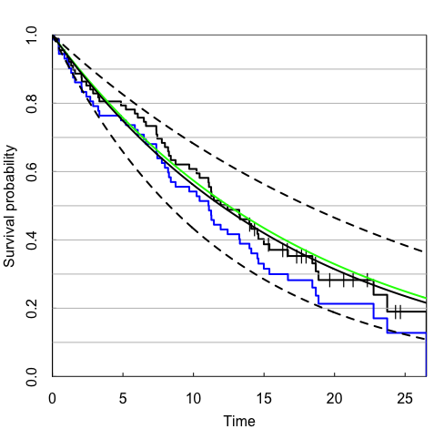
The results are plotted in Figure 1. The black step function is the adjusted Kaplan-Meier estimate, with censored observations denoted by vertical tick marks. The green curve is the true survival function for the patients randomized during the last year of accrual. The smooth black curve is the Bayesian model estimate of the survival function for these patients, and the two black dotted curves are 95% credible intervals.
For reference, the standard Kaplan-Meier estimate is also shown in blue. By treating the older observations as if they had the same hazard rate as the newer, this approach underestimates the survival function for the newer data.
In our experience, the adjusted Kaplan-Meier estimates tend to overlap nicely with the estimates of the survival curve from the Bayesian model: both are adjusted using the same estimated hazard ratios. Unadjusted Kaplan-Meier plots can appear to diverge from model estimates even when there is only weak evidence of a time trend.