Introduction
Purpose of this document
This document describes how use the FACTS Dose Escalation (DE) 2D-CRM design engine. It is intended for all end users of the system.
Scope of this document
This document covers the FACTS Dose Escalation 2D-CRM design engine user interface.
This document does not address the internal workings of the design engines or algorithms, which are addressed in the associated Design Engine Specification. It also does not address the use of FACTS Core Designs or Enrichment Designs, which are covered in other User Guides.
The screenshots provided are specific to a particular installation and may not reflect the exact layout of the information seen by any particular user. They were taken from FACTS 6 or later installed on Windows 10. Different versions of Windows or the use of different Windows themes will introduce some differences in appearance. The contents of each tab, however, will be consistent with the software.
Citing FACTS
Please cite FACTS wherever applicable using this citation.
FACTS 2D-CRM Overview
This user guide assumes some limited general familiarity with FACTS and concentrates on describing the interface for designs using the 2D-CRM approach. See the FACTS Dose Escalation user guide for a general introduction to the FACTS Dose Escalation user interface.
The 2D-CRM is based on the method described in the paper (Neuenschwander, Branson, and Gsponer 2008). It is designed for use in oncology phase 1 trials, and we understand has been used at Novartis for some trials of this type:
Combinations of doses of two drugs are to be tested.
Dosing starts at a (very) low dose combination, strongly believed to be safe.
Usually after a cohort of subjects have completed their current dose, the dose to be used for the next cohort is selected. The selection of this dose is dictated by a combination of dose escalation rules, the estimate of the toxicity rate on the different doses and the target maximum tolerated toxicity, or toxicity band.
The endpoint per subject is binary: toxicity observed or not.
There are two predefined sets of doses to explore, one for each drug. Not all combinations may be permitted.
There is limited sample size.
FACTS 7.0
There have been no changes to 2D-CRM in FACTS 7.0.
FACTS 6.5
There have been no changes to 2D-CRM in FACTS 6.5.
FACTS 6.4.1 Changes to 2D-CRM
Compared to 6.4 there have been slight changes to address circumstances where the model could fail to converge, and parameter estimates could reach very large values. This was due to wanting to allow 0 doses in 2D-CRM, because in the 2D setting it is sometimes the case that there have been monotherapy escalation studies and there is a desire to incorporate this data in the 2D trial. To do this a 0 dose is included for the other drug so there are monotherapy combinations in the design (possibly excluded from being actually given during the 2D trial). This means the posterior parameter estimates from the monotherapy can be used for that drug’s prior, or the data from the monotherapy trial can be included as “Prior Toxicities”.
Up to this release (6.4.1) there were two problems doing this:
Inherited from the N-CRM code, FACTS was still storing the logs of the dose strengths, so doses could not be 0, and the advice was to use small values instead such as 0.001.
The presence of a combination with very small values for the transformed dose strength (and now 0 values) causes problems for the model’s stability, in particular when the dose strengths are 0 it becomes impossible for the model to have anything other than 0 DLT rate at the 0,0 combination.
In FACTS 6.4.1 these problems have been addressed by the following changes:
FACTS now allows 0 strength doses.
It there is any combination where both dose strengths after transformation are less than 0.001 then this combination must be excluded from the trial and can have no prior toxicities specified for it (however prior observations of no toxicities are allowed).
If both drugs include 0 strength doses, the lower asymptote for the Response Model (the range is usually [0, 1]) must be raised slightly, e.g. to 0.0001.
Restrictions 2 and 3 are checked when there is an attempt to run simulations, and if violated a warning message is displayed and the simulations not run.
FACTS 6.4 Changes to 2D-CRM
There were no changes to the 2D-CRM simulator for FACTS 6.4.
FACTS 6.3 Changes to 2D-CRM
There were no changes to the 2D-CRM simulator for FACTS 6.3.
The use of the 2D-CRM simulator to design a trial
The typical pattern of use of the simulator is as follows:
Enter the constraints and objectives of the study: maximum sample size and the bounds of the different toxicity bands.
Select the choice of and overdose control thresholds.
Specify a small number of expected toxicity responses as VSR scenarios.
Select the desired run-in and dose escalation rules.
Specify an initial set of priors for the model.
Run a small number of simulations (25 is usually adequate at this stage) of each scenario.
Check the performance of the design:
Do the majority of the final combinations being selected have an acceptable level of toxicity?
Is the overall level of toxicity observed in the trial acceptable?
In the scenarios where the performance is worst, observe the behavior in individual simulations.
Try a number of modifications to the design and simulate each modification individually. Increasing the number of simulations (usually 100 is still adequate at this stage).
Consider if more VSRs need to be included to check a greater range of possible actual toxicity rate patterns.
Combine modifications with promising results and re-simulate, (usually 500 is an adequate number at this stage).
The design changes that are typically considered are:
Exclude low dose combinations that are certain to be too weak.
Exclude high dose combinations that are certain to be too toxic.
Modify the run-in to be more aggressive if it is taking too many subjects and cycles to reach the escalation phase.
The ”Huang” diagonals method is the least aggressive, both the “Ivanova” and “Tri-axial” can skip some combinations, finally consider a user specified run-in sequence.
The “Huang” and the “Tri-axial” can make use of the “multiple simultaneous cohorts” option in the run-in phase to test multiple combinations simultaneously.
If the escalation phase is too aggressive – incurring too many toxicities or selecting combinations with high toxicity true toxicity too often - then options are:
Make the run-in expand at the dose below observed toxicities, not at the toxicity
Make the priors for the model less informative (if the priors are informative and predicting low toxicity at higher combinations), the greater uncertainty in the toxicity at higher doses may then result in the estimate of their toxicity exceeding the overdose control threshold.
Make the priors for the model predict higher levels of toxicity.
Increase the overdose control thresholds.
Shift the toxicity band bounds downwards.
Add prior toxicity data.
Increase the number of subjects before escalation.
If the escalation phase is not aggressive enough – selecting combinations with too low a toxicity too often - then options are:
Make the run-in expand at the dose where toxicity observed not a dose below
Make the priors for the model more informative (if the priors are uninformative) this will allow lack of toxicity on lower doses reduce the predicted toxicity at higher, untested doses, bringing the probability of toxicity at the higher doses below the dose escalation threshold.
Make the priors for the model predict lower levels of toxicity.
Lower the overdose control thresholds.
Shift the toxicity band bounds upwards.
Add prior toxicity data.
Decrease the number of subjects before escalation.
General constraints and assumptions
The design engine is limited to phase 1/2a designs with dichotomous endpoints toxicity/no-toxicity. There is no longitudinal modeling or analysis of covariates included. All results of a cohort are assumed to be available before the next cohort is treated.
Models and Methods
For a full description of the models and methods implemented in the 2D-CRM see the Software Specification document [Spec].
In the current version there is a single statistical model used to analyse the data – the 5 parameter Bayesian Logistic Regression Model as described in (Neuenschwander, Branson, and Gsponer 2008). The model is used to compute the posterior probability that the toxicity rate at each combination is in one of 4 toxicity bands – “underdosing”, “target toxicity”, “excess toxicity” and “unacceptable toxicity”. The boundaries between the bounds are settable by the user.
The posterior probability that the rate is in the target toxicity rate is used to target the dose allocation – the method attempts to allocate to the Maximum Target Toxicity (MTT). The posterior probability that the rate is in the “excess toxicity” and “unacceptable” or just the “unacceptable” bands can be used to enforce an “overdose control”. Combinations with a posterior probability that exceed the specified threshold are excluded from selection or allocation.
The dose combinations are explored in two phases:
Optionally the trial may begin with a “small cohort run-in” or the allocation of a single cohort to a specified combination. This phase ends when the sequence of combinations to explore is exhausted or excluded by combinations at which toxicities have been observed. There is no model fitting during this phase.
The trial then proceeds looking for the dose combination with the highest probability of having a toxicity rate in the target toxicity range using dose escalation, limited by dose escalation rules.
Run-in methods
There are 4 run-in methods available:
- Contour
- This explores the reverse diagonals, assuming that the expected toxicity at the dose increments of the two doses are roughly equal.
- Row by row
- This explores the doses of drug 1 at the first dose of drug 2, then increments drug 2, steps back a specified number of doses in drug 1 and then increments through the doses of drug 1 again. This method favours escalation of drug 1 over escalation of drug 2.
- Tri-axial
- This explores the combinations on each axis and on the diagonal. For small numbers of dose increments it is similar to the Huang run-in. For larger numbers of dose increments it is more parsimonious.
- Custom
- This explores a specific sequence of combinations stopping when the first toxicity is observed or the sequence is completed.
Or run-in can be skipped.
For more details see the Software Specification document [Spec].
Escalation methods
There are 4 escalation methods available. They all work in the same basic framework:
The dose combinations where sufficient subjects have been tested and lesser dose combinations are found.
The dose combinations that can be escalated to beyond these are found.
The dose combinations where the overdose control limits are exceeded are removed.
The target dose combinations from the remaining set are selected according to the selected method.
The 4 methods are:
- Contour
- This explores every MTT on every row and every column (frequently these overlap, but not necessarily).
- Walk
- This explores the MTT that is at or adjacent to the last combination tested (excluding the dose that is an increment in both drugs from the last combination tested).
- Tri-axial
- This explores the MTT on each axis and on the diagonal. Once these have the required maximum subjects on MTT, any combinations off the axis and diagonal that are the MTT are explored.
- Allocate MTT
- This allocates to the combination that is the overall MTT of all the combinations that it is permitted to allocate to.
Outstanding Issues / Absent Features
Currently the most obvious absent features are:
modeling of additional endpoints such as efficacy or drug exposure
the modeling of ordinal toxicity
the simulation of open enrolment where subjects are allocated on subject by subject basis as they become available for enrolment, with a limit on the number of subjects who can being treated but for whom final endpoint has not been observed.
The FACTS 2D-CRM GUI
The FACTS 2D-CRM GUI conforms to the standard FACTS GUI layout, with information and displays divided across various standard tabs (Figure 1).
The Study Tab has sub-tabs for entering Study Information and specifying the Treatment Arms (doses) available in the study. This is where the user specifies the ‘given’ requirements, or constraints, of the trial to be designed.
The Virtual Subject Response tab has sub-tabs for specifying Explicitly Defined response scenarios to simulate and loading External data files of simulated subject responses. This is where a set of different toxicity rates per dose are specified that should represent the expected ‘space’ of the expected dose-toxicity profiles for the compound being tested.
The Design has sub-tabs for specifying the Start-up phase, the Dose Escalation phase, the Toxicity Response model and any prior toxicity data to include. These are the design choices open to the trial biostatistician. The expected consequences of these design choices are estimated by running simulations of the trials using the various virtual subject response profiles defined.
On the Simulation Tab, the user controls and runs simulations and can view the simulation results.
On the Analysis tab, the user can use the design to analyze a specific data set and report the result of fitting the specified toxicity response model and the recommended dose for the next cohort.
Also on the menu bar, on the right hand side of the FACTS Window, is a button labeled “Notes”; clicking this button reveals a simple “notepad” window in which the user can maintain some simple notes that will be stored within the “.facts” file.
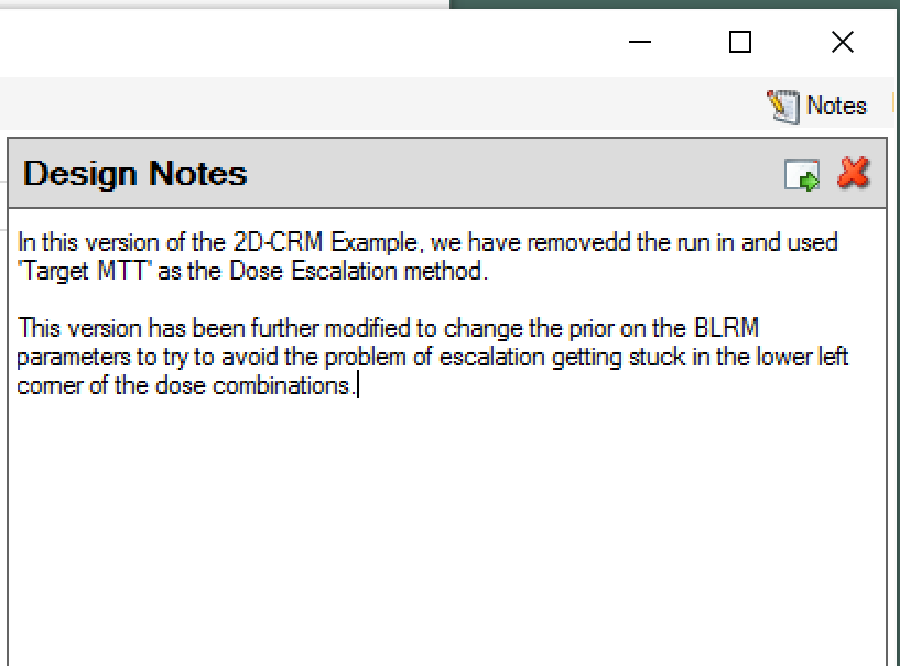
The notepad window comes with two further buttons: one to change the window to a free floating one that can be moved away from the FACTS window; and the other to close it.
The Notes field can be used for any text the user wishes to store with the file. Suggested uses are: to record the changes made in a particular version of a design and why; and to comment on the simulation results. This will help when coming back to work that has been set aside, to recall what gave rise to the different version of a design.
The Study Tabs
Study Info
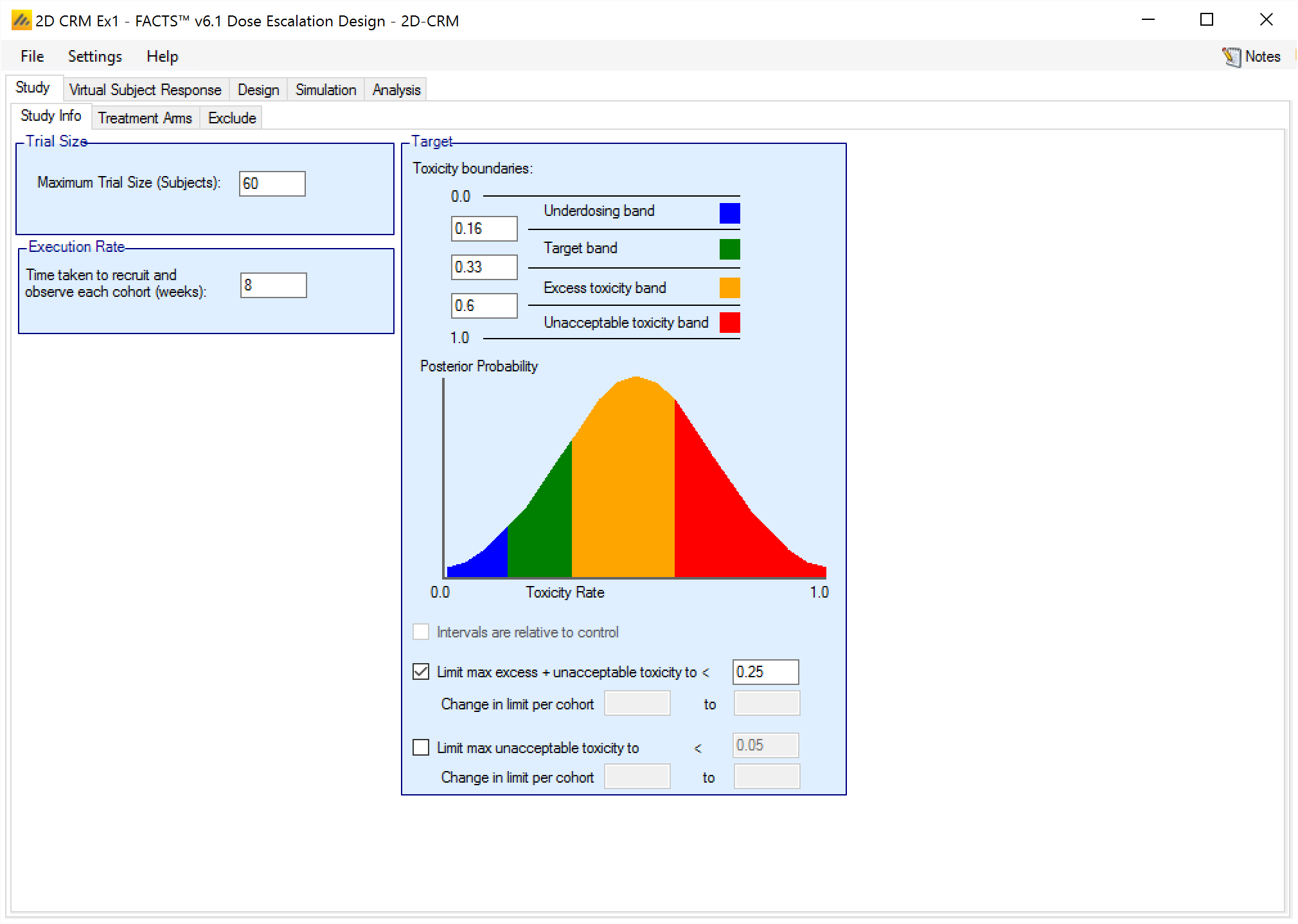
On the Study Info tab the user can
Specify the maximum trial size (in subjects not cohorts, as subjects tested in the run-on phase count to the overall total).
Specify the parameters of the target, the user specifies the boundaries between the different toxicity bands, and whether using overdose limits and if so which ones and what the overdosing thresholds are.
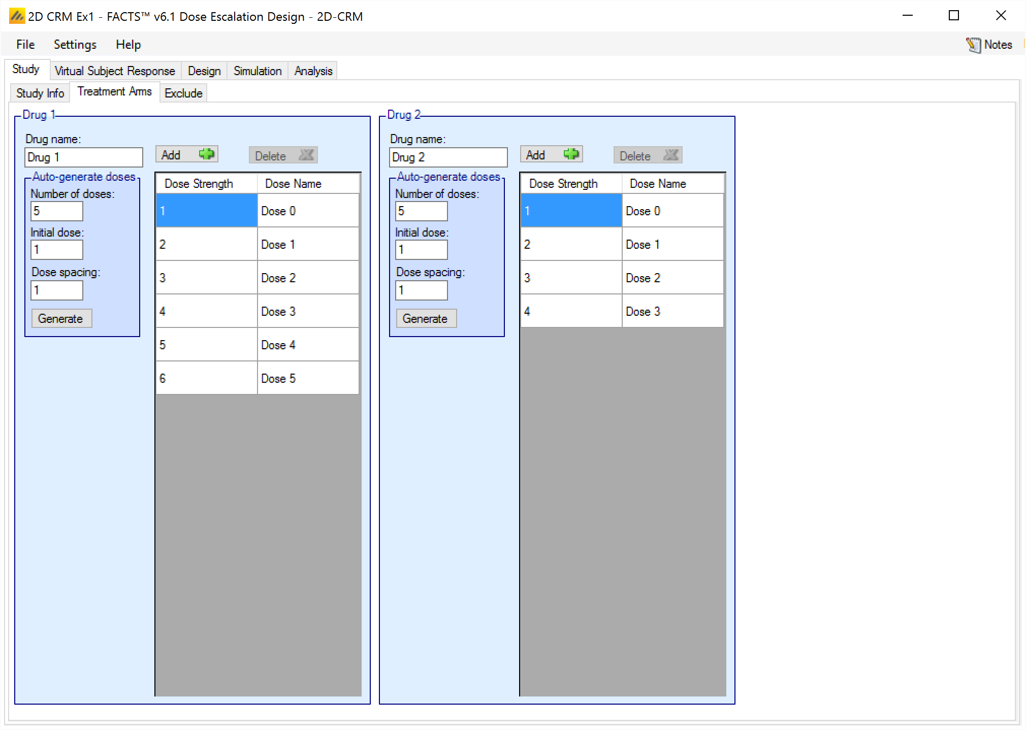
Treatment Arms
On the Treatment Arms tab the user specifies the names of the drugs, and the number, relative strength and names of the doses of each drug. The user can either click the ‘Add’ button the required number of times or use Auto generate doses, specifying the number of doses to create and initial dose level. Auto generate deletes all the pre-existing doses before generating the new ones.
After creating the desired number of entries the user can edit the strengths and names of the doses.
It is up to the user to ensure that the dose strengths are in monotonically increasing order.
It is now (FACTS 6.4.1 and later) possible to enter dose strengths of 0, to create dose combinations that are monotherapies. This is particularly useful for enabling prior information from monotherapy trials to be included in this design.
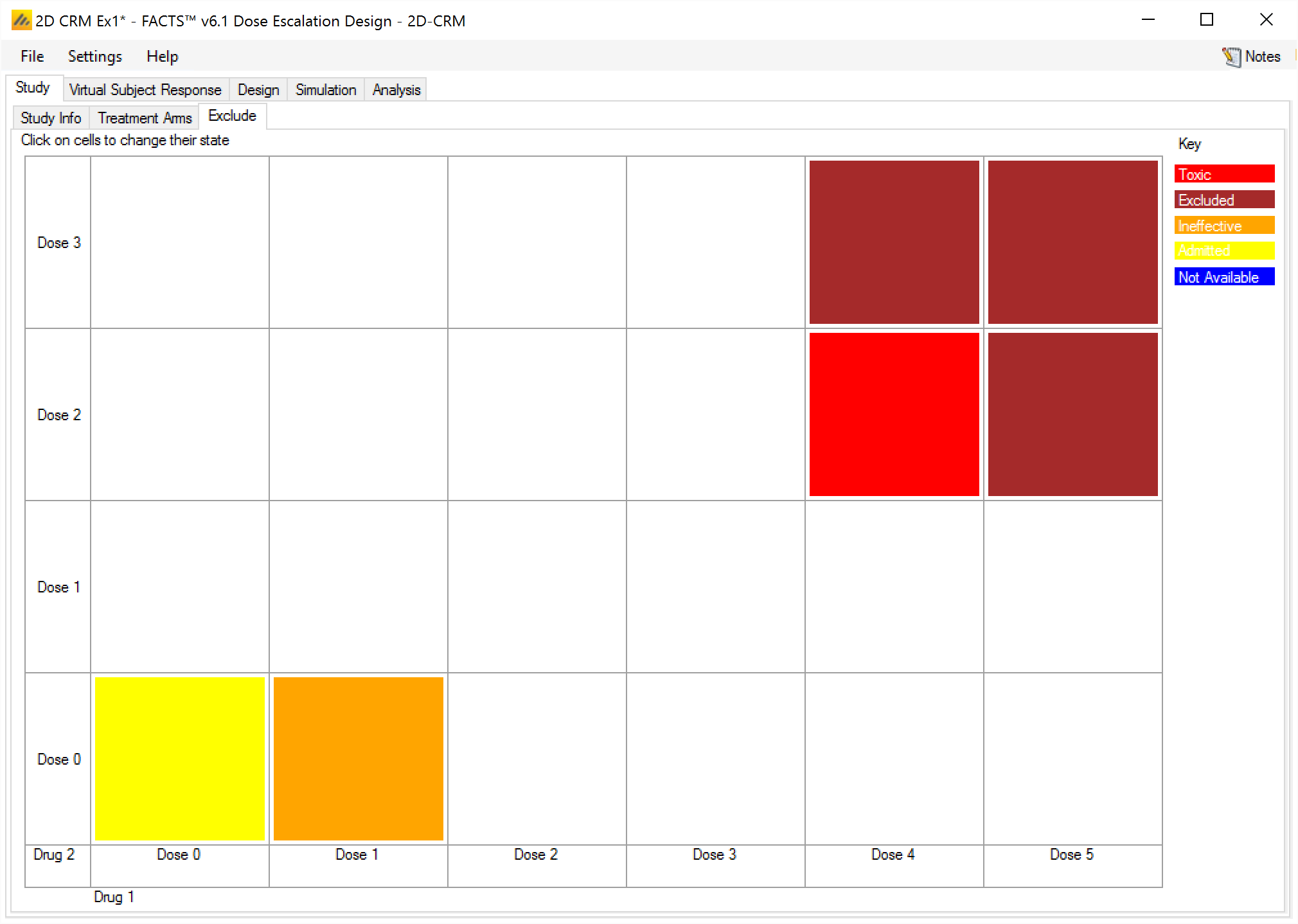
Exclude
On the Study > Exclude tab the user can specify dose combinations that cannot be used in the trial. By clicking on any square on the grid the corresponding dose combination is cycled through the following states: ‘Toxic’, ‘Not Available’, ‘Ineffective’ and ‘Available’. The initial state is ‘Available’ for all combinations.
If a combination is specified as ‘Toxic’ then all the combinations where both drugs are at the same or higher strength are also excluded.
If a combination is specified as ‘Ineffective’ then all combinations where both drugs are at the same or lower strength are also excluded.
If a combination is specified as ‘Not Available’ then just that combination is excluded with no consequences for the combinations around it.
If there are any combinations where, after transformation of the dose strengths, both drugs have a dose strength of less than 0.001 this must be excluded from the trial (mark them “ineffective” or “not available”). Any toxicities occurring on such a combination would be data that the model would have difficulty fitting.
The Virtual Subject Response Tabs
The Virtual Subject Response tabs are used to define the toxicity rates to use in simulating subjects responses. In each scenario a specific toxicity rate is specified for each dose combination. Thus a range of different scenarios is usually created that span the range of toxicities that are believed credible. As well as the absolute toxicities the scenarios should span the different rates at which its thought that the toxicity rates could change from dose to dose, and also span the different degrees of drug-drug interaction – both +ve and –ve that are believed credible.
There are two ways of specifying scenarios: Explicitly entering the rate to simulate for each combination, and Parametrically entering the parameters of a simple model from which the toxicity at every combination then derived.
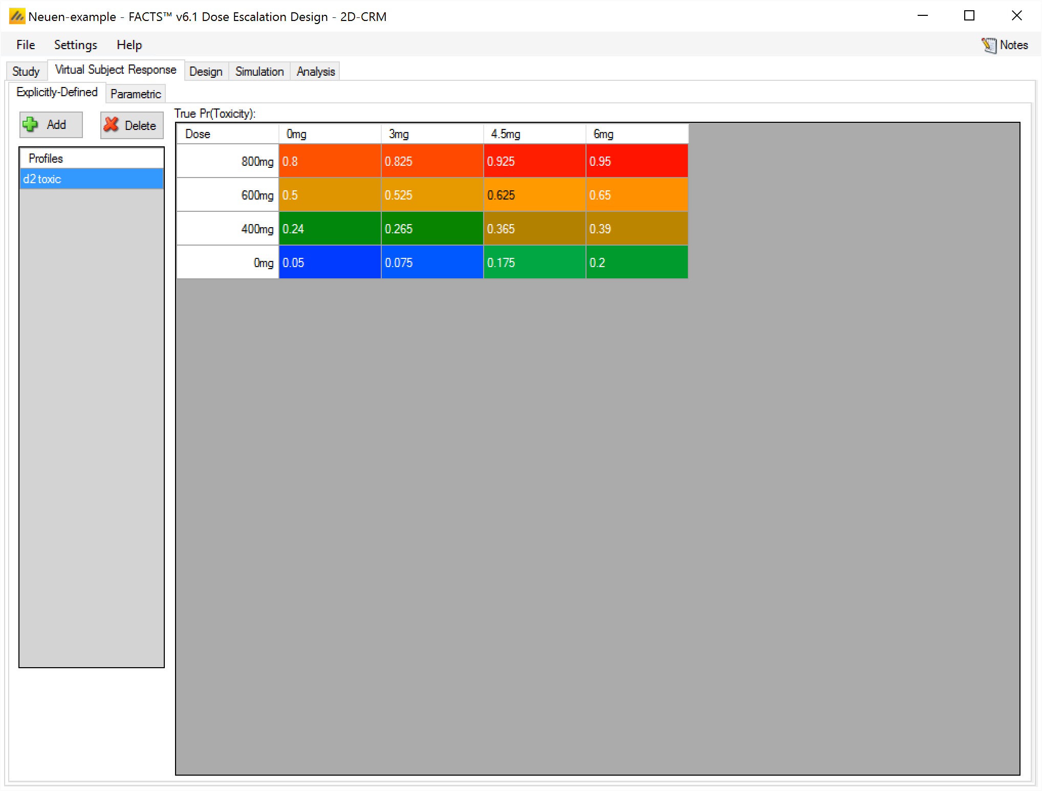
Explicitly Defined
On the VSR > Explicitly Defined tab, the user enters the toxicity rate to use when simulating subject responses, for every dose combination. The cells are colored according to the toxicity band coloring convention used in FACTS (under-dosing: blue, target: green, excess: orange, unacceptable: red) according to the toxicity rate entered.
Parametric
On the VSR > Parametric tab, the user enters the parameters for a model that generates a toxicity rate to use when simulating subject responses, for every dose combination. The cells are colored using toxic band coloring according to the toxicity rate of that dose combination.
The model used is the 5 parameter BLRM model that is used as the Toxicity response model on the Design > Response Model tab, but the user can specify different ‘effective dose strength’ models from those used in the analysis.

For each profile the user specifies:
For each drug the ‘effective dose strength’ model.
The reference dose (where the effective dose strength is 1 and the toxicity rate due to that drug is given by the Alpha parameter alone).
Whether the effective dose strength is the ratio of dose strength to the reference dose or the exponential of the difference of the to dose strength from the reference dose.
For each drug the values of the coefficients of the single drug models entered as ln(alpha) and ln(Beta)
The value of Eta, the drug-drug interaction term – Eta is the log-odds ratio between the interaction and the non-interaction model at the reference dose combination.
It is perfectly reasonable to use the parametric models by simply varying the parameters using trial and error until the desired set of toxicity rates is achieved.
The Design Tabs
The Design tab allows the user to specify:
Start-up: where the parameters of the run-in phase (if any) are specified.
Dose Escalation: where the ad hoc rules for limiting dose escalation and early stopping are specified.
Response Model: where the priors for the dose-toxicity model are specified.
Prior Toxicities: where any prior observations are specified.
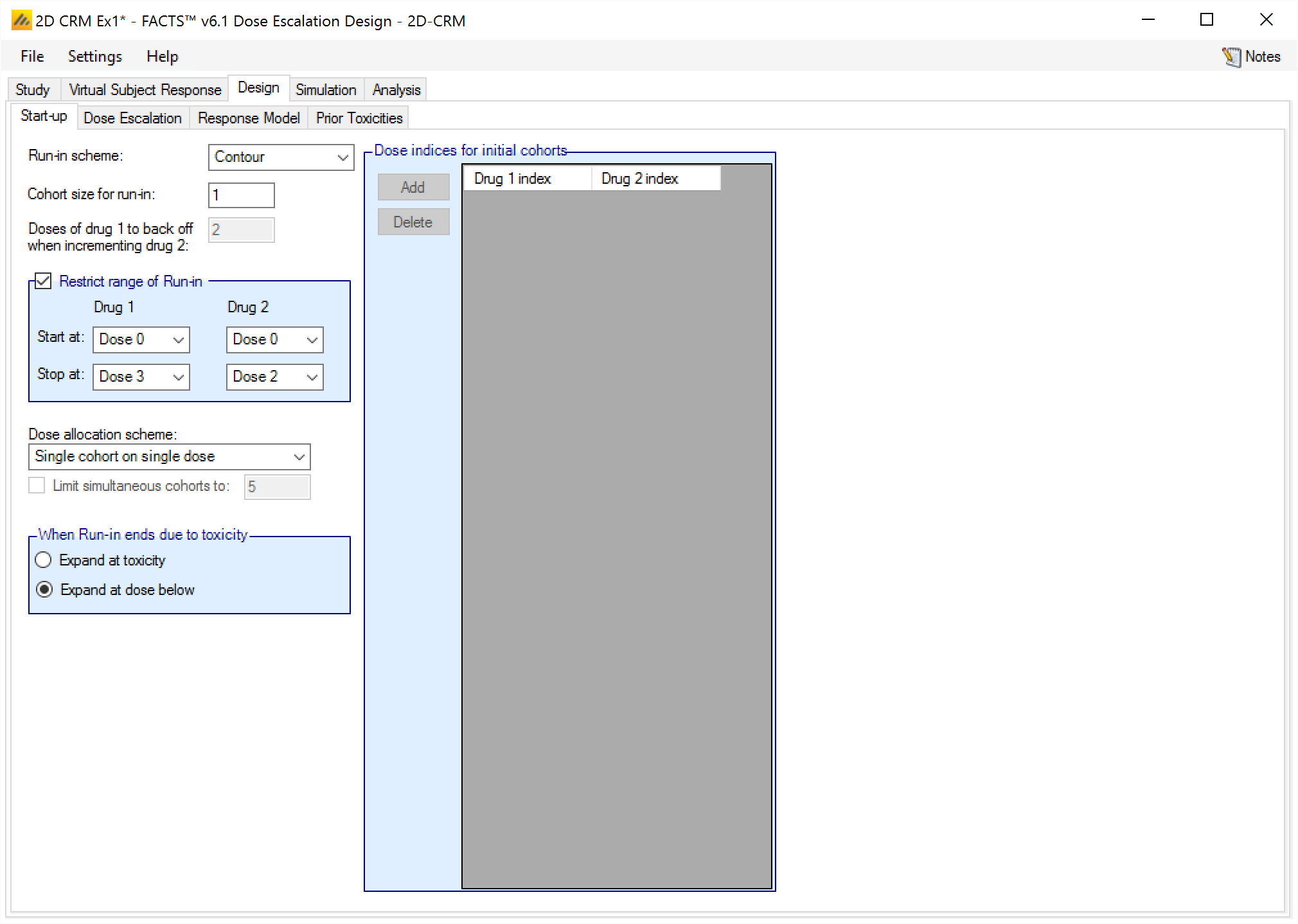
Start-up
The Start-up tab allows the user to specify what is commonly referred to as a single patient run-in, in the FACTS 2D-CRM it’s allowed to be a “small cohort“ run-in. (The paper (Ivanova et al. 2003) showed that smaller target toxicity rates benefited from larger cohort sizes in the run-in).
On this tab the user can specify
The scheme to use for the run-in: “None”, “Contour”, “Row by Row”, “Tri-axial” or “Custom”. These are described above and in [Spec].
- If “None” is specified then the table for specifying specific dose combinations is used to specify the dose combination(s) to be assigned to the starting cohort(s). These will be the full sized cohorts used in the escalation phase.
The cohort size to use in the run-in. A size of ‘1’ yields a ‘single patient run-in’, but other values are possible and may give better results, (see (Ivanova et al. 2003)).
For the ‘Row by row’ run-in scheme, the number of drug 1 dose increments to back-off each time drug 2 is incremented.
The range of the run-in. If the user does not want the run-in to possibly run all the way up to the maximum dose strengths, even if no toxicities have been observed, it is possible to specify a rectangular area of dose combinations for the run-in to include by specifying the starting combination (the lower left corner of the rectangle) and the stopping dose (the upper right corner combination). Note that as you would expect, regardless of whether this feature is used or not, dose combinations that have been excluded from the study on the Stud > Exclude tab are excluded from the run-in.
The dose allocation scheme: (only applies to the Contour and Tri-axial run-in schemes):
allocate a single cohort;
allocate the cohort across the next possible dose combinations;
or allocate a cohort to each of the next dose combinations and optionally specify a maximum number of cohorts / dose combinations that can be tested at a single step.
The Row by row and Custom run-ins only identify one dose combination to test next, and so use “single cohort” allocation regardless of the setting of this control.
Where to allocate after the end of the run-in it it ends due to observing toxicities, either:
expand the allocation at the combinations where toxicity has been observed,
or at one dose increment below where toxicity has been observed.
If the run-in ends because it has reached the end of the combinations to be tested during run-in without seeing a toxicity, then dose escalation starts by expanding at the allocation of the maximum dose combination(s).
- If use of a Custom run-in has been specified, then the sequence of dose combinations is specified.
Dose Escalation
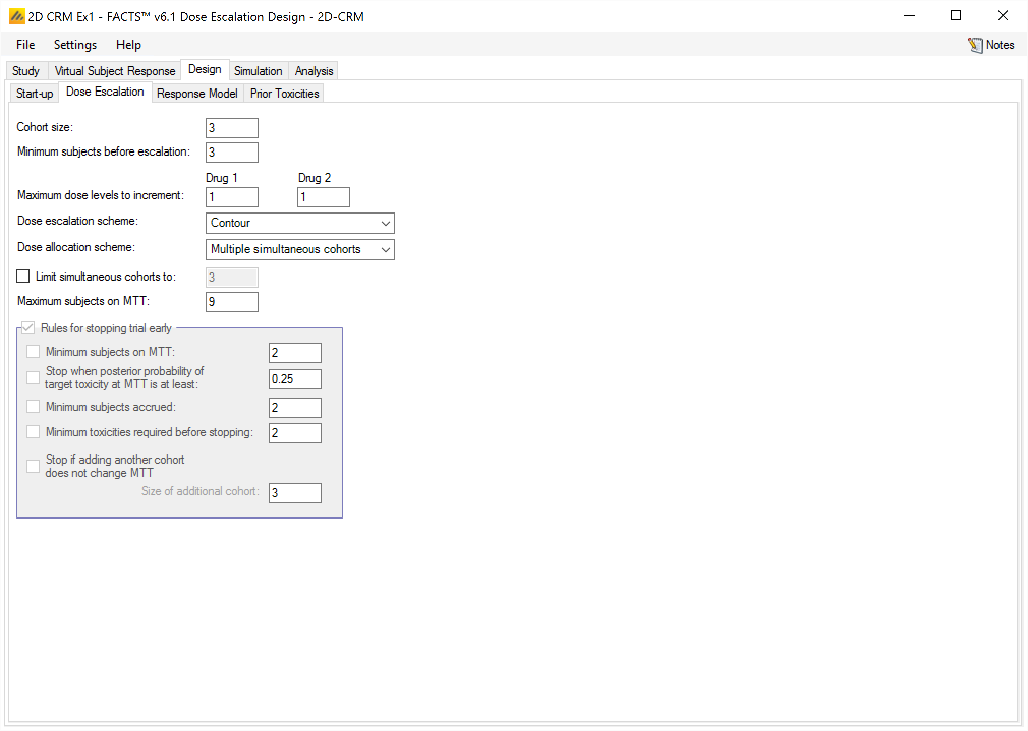
The Dose Escalation tab allows the user to specify the dose escalation and early stopping rules to use during the Dose Escalation phase.
On this tab the user can specify:
The cohort size.
The minimum number of subjects: that must be have been tested at a combination before the trial can escalate to a higher dose combination (that is not excluded by the overdose control).
The maximum dose increment: in either drug that can be applied from a combination that has been tested, and where the minimum of subjects have been tested, to a higher dose combination.
The dose escalation scheme: “Contour”, “Walk”, “Tri-Axial” or “Allocate to MTT”. These are described in (2.3.2) and in [Spec].
The dose allocation scheme: (only applies to the “Contour” and “Tri-axial” schemes):
allocate a single cohort;
allocate the cohort across the next possible doses;
or allocate a cohort to each of the next doses.
The “Walk” and “Allocate to MTT” escalation schemes only identify one next combination, and so use “single cohort” allocation regardless of the setting of this control.
If “Multiple simultaneous cohorts” is specified, then it is possible to set a limit on the maximum number of cohorts / dose combinations tested in the next step.
- Maximum subjects on MTT. This is the maximum number of subjects to allocate to a combination under Dose Escalation. In the “Contour”, “Walk”, “Tri-Axial” escalation schemes this is currently the only stopping rule. If all the targeted combinations have the maximum number of subjects on them, the trial stops.
All the escalation schemes stop if the maximum number of subjects has been allocated or all combinations are too toxic (the posterior probabilities of toxicity exceed the overdose threshold). The schemes other than “Allocate to MTT” can also stop when the maximum number of subjects on MTT is reached on all the target doses.
If the “Allocate to MTT” escalation scheme, is being used then additional stopping rules similar to those available in N-CRM can be enabled. If they are enabled, then the following may be specified:
Minimum subjects on MTT: the trial can only stop with a combination selection if the combination to be allocated to have at least these number of subjects on them.
Stop when Posterior Probability of target Toxicity at MTT is at least: the trial can stop with a combination selection when the combination to be allocated to has a posterior probability that its toxicity rate is in the Target Toxicity band is at least the specified amount.
Minimum cohort’s accrued: the trial can only stop with a combination selection if the specified minimum number of cohorts has been allocated and completed.
Minimum toxicities: the trial can only stop for all combinations too toxic if the required minimum number of toxicities have been observed. Whilst all combinations are too toxic but this minimum number of toxicities havs not been observed, subjects are allocated to the lowest dose combination.
Response Model
The Response Model tab displays a description of the model and 4 other components:
- A panel where the prior distributions for the model parameters can be input. Unless prior toxicity information is also to be included, it is recommended that uninformative priors are not used as these tend to lead to a failure to re-escalate to a dose if just one toxicity has been observed there, due to overdose control.
Values that represent weakly informative priors are recommended instead. The prior mean and SD for each Alpha should represent the prior expectation (in log-odds) of toxicity at the reference dose for that drug in isolation. Having set Alpha the prior for Beta should be set to allow gradients that are as steep as plausible, but if set too high, or too broad it may cause problems of not being able to escalate to high doses because of overdose control (even with few toxicities at low doses the uncertainty of the model at higher doses where there is currently no data may mean the posterior estimates of toxicity at these doses exceed the overdose control thresholds). This can be checked looking at example simulations or manually by entering test data on the Analysis tab. The prior for the correlation should usually be zero or slightly negative. A positive prior for Rho means that if the value for Alpha is estimated as low (due to low toxicity being observed near the reference dose) then the value of Beta will be estimated as being low – and this may lead to too low an estimate of toxicity at higher doses. A very strongly negative prior for Rho can lead to the same problems as a too high or broad prior for Beta.
- A panel where the transformations of the virtual dose strengths to values that can be used by the model is specified. This transformation is usually the dose ratio of each dose to the median dose of that drug. Options to use a linear transform and a different reference dose are available.
The recommended values for the reference dose are either the center of the dose range (the default “Median dose”) or the dose thought most likely to be in the middle of the target toxicity range for that drug alone.
- Re-scaling the response model. The model estimates rates between 0 and 1 and works best when the observed rates are asymptotically 0 or 1. If the observed toxicity is known to have different minimum and maximum rates (0.1 and 0.5 say) then the model fits is much, much better if these are specified as the asymptotes in place of 0 and 1.
If a dose combination of 0,0 is included in the design (even when excluded from be used in the trial, as it must be) the response model must be re-scaled with a minimum asymptote above 0, even if only very slightly (such as 0.0001).
- The last panel displays the values of the model at the dose combinations using the specified parameters.
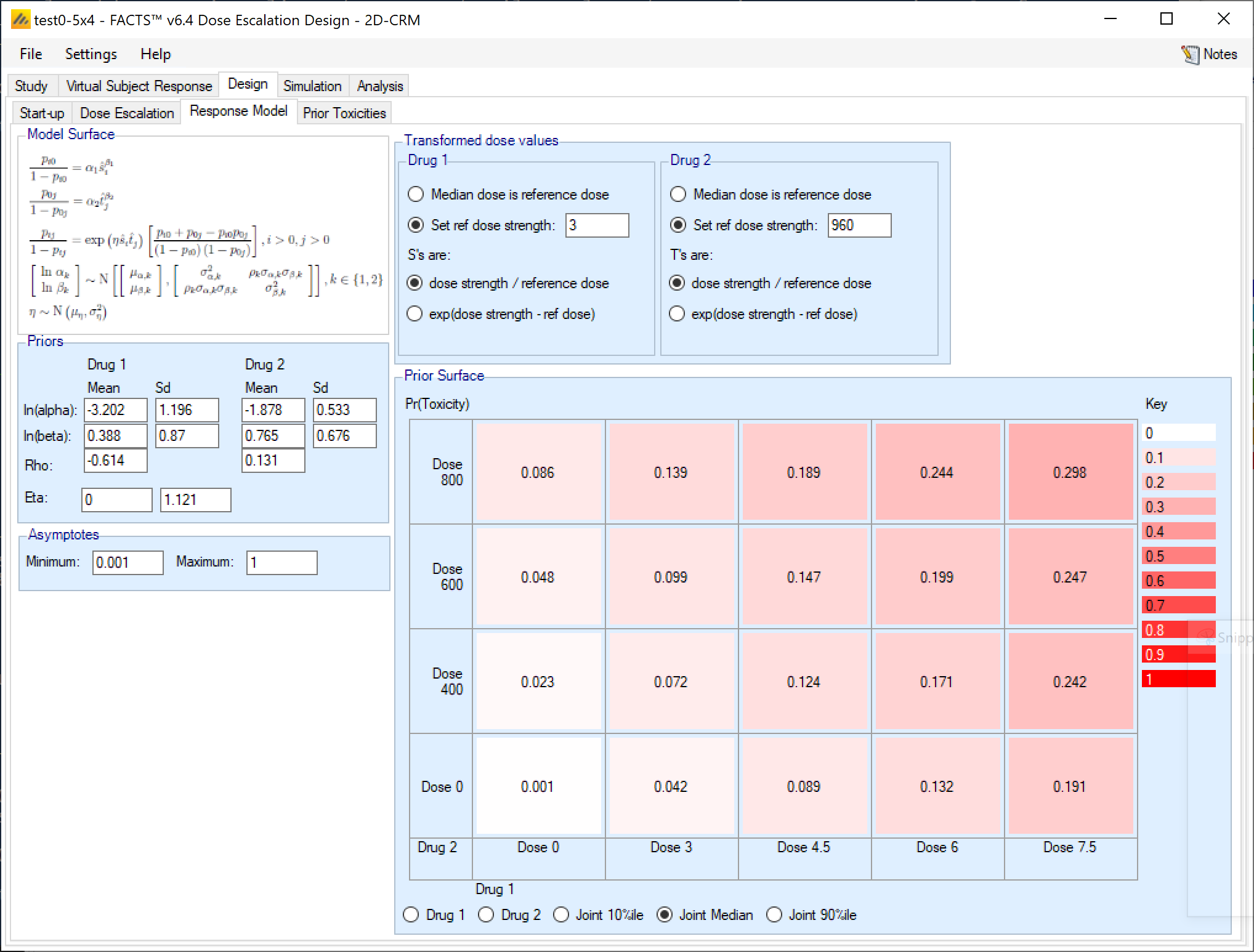
Specifying the Priors: The priors for each pair of parameters (α,β) for the response model for each drug are specified via a bivariate normal distribution (as in the single drug N-CRM), with a separate mean and SD for α and β, and a correlation term ρ (Rho). The prior for the interaction term η (Eta) is the mean and Sd of a Normal distribution. Using a Normal prior for Eta allows Eta to be -ve, modeling a negative interaction between the drugs and resulting in a non-monotonic surface. Unless a negative interaction is thought possible, it is recommended that the lognormal prior for Eta is used
Specifying the dose transform: For both drugs the transformation of the dose strengths to a range of values suited to the model is specified. For each drug the transformations are relative to ‘reference’ dose, by default the median value in the dose range. The transformation can be linear log(d – d*) or the dose ratio ((d/d*))
Specifying the asymptotes: The model fits values in the range (0-1), asymptotically approaching either limit. If desired the range can be reduced by re-scaling so that it asymptotically approaches a specified lower limit > 0 and upper limit < 1.
Checking the prior: The influence of the prior on the model can be checked by viewing the results of sampling of the model parameters from the specified prior. Options are to view a) 100 samples of the 1-dimensional model for drug 1 or drug 2, or b) 1,000 samples of the 2-dimensional model over both drugs showing the 10%-ile, median or 90%-ile toxicities at each dose combination.
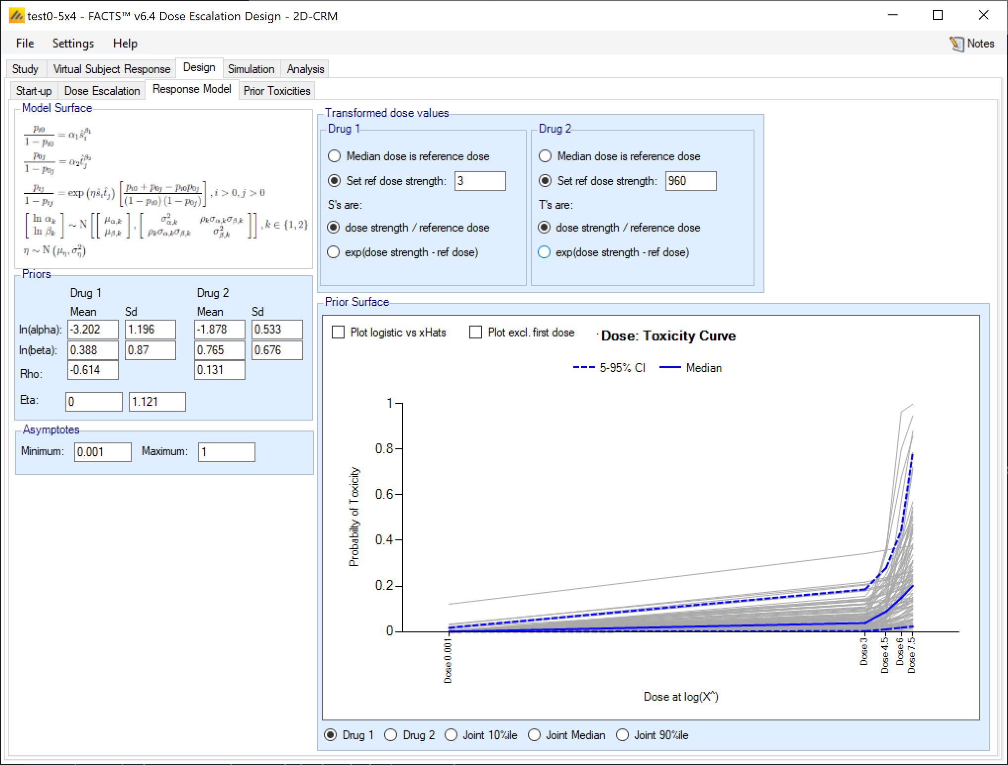
The individual drug graph plots the doses at the log of their transformed dose strength (“Log(X^)”), this enables the logits to be plotted linearly.
If there is a transformed dose strength of 0, this is plotted at some notional value that represents -infinity, and to see the plot at the other doses the “Plot excl. first dose” option should be checked.
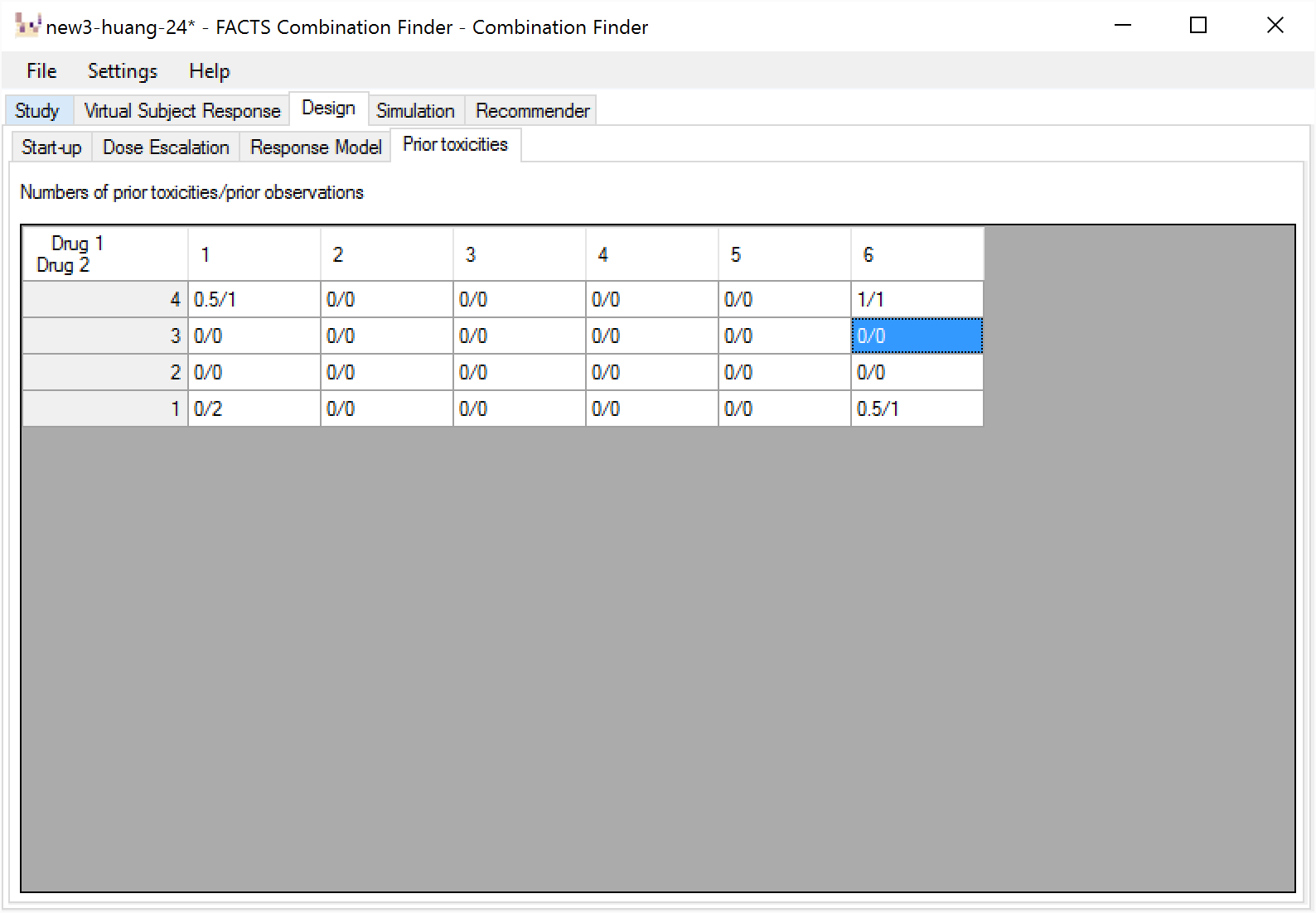
Prior Toxicities
This tab allows prior information to be included with the data collected during the trial.
The user can specify, for any dose combinations a prior observed number of toxicities and number of observations. To allow the prior data to be down weighted, the user is allowed to enter fractional amounts.
The specified prior data is simply added to the observed data when fitting the model, but this is logically equivalent to fitting the model with the specified prior to the specified prior data and then using the resulting posterior estimate of the model parameters as the prior for fitting the model to the observed data.
Some idea of the effect of the prior data can be gained by using the “Analysis” tab, and performing an analysis on a dataset without any additional subject data.
If there is a combination where the transformed dose strengths of both drugs are below 0.001, there can be no prior observed toxicities for that combination (it would be impossible for the model to fit them).
Simulation Tab
The Simulation tab allows the user to execute simulations for each of the scenarios specified for the study. The user may choose the number of simulations, whether to execute locally or on the Grid, and modify the random number seeds.
If completed results are available, the actual number of simulations run for each scenario is reported in one of the first columns of the results table. The value displayed in the “Number of Simulations” control is the number of simulations that will be run if the user clicks on the ‘Simulate’ button.
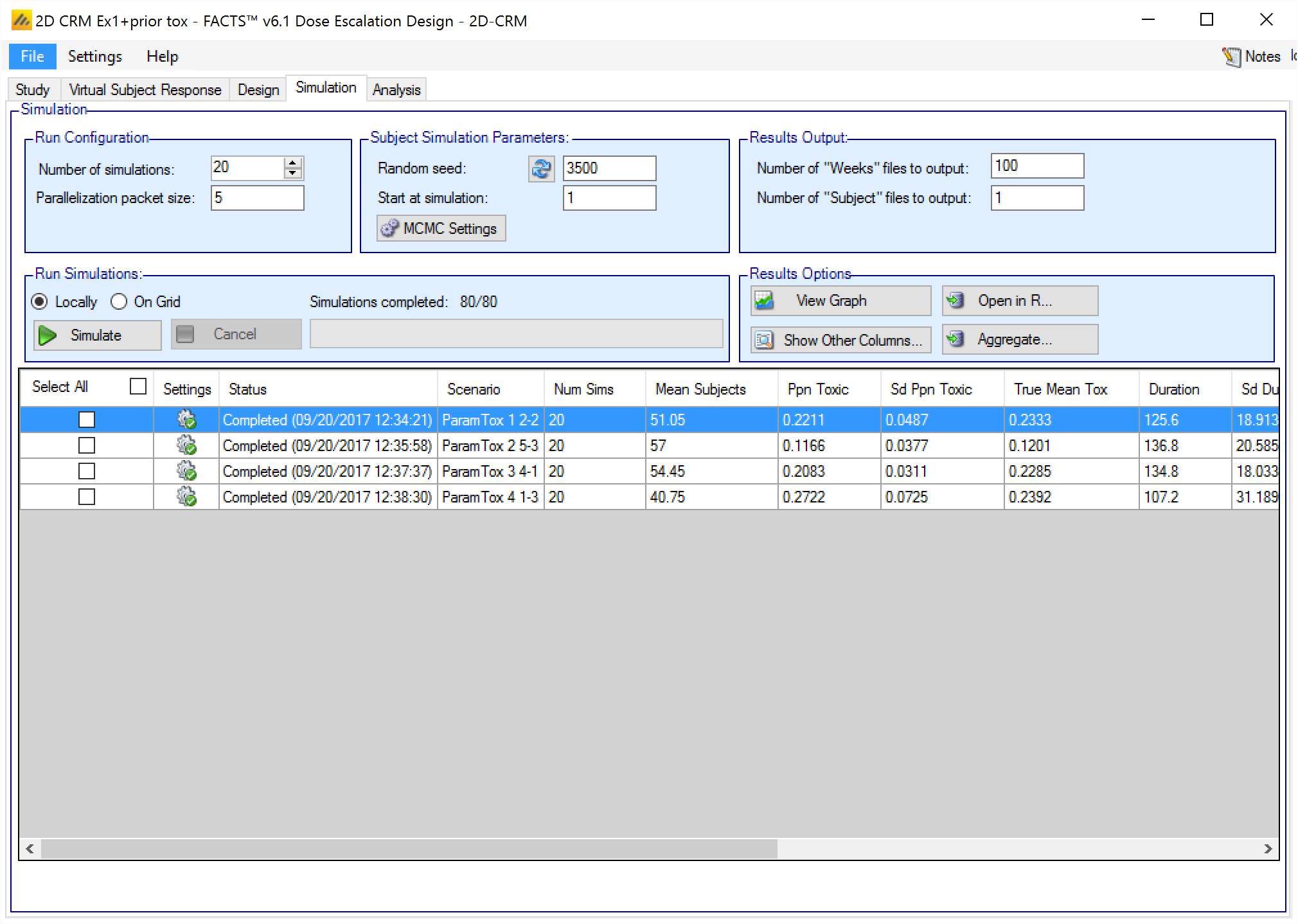
FACTS uses Markov Chain Monte Carlo methods in the generation of simulated patient response data and trial results. In order to exactly reproduce a statistical set of results, it is necessary to start the Markov Chain from an identical “Random Seed”. The initial random seed for FACTS simulations is set from the simulation tab, the first thing that FACTS does is to draw the random number seeds to use at the start of each simulation. It is possible to re-run a specific simulation, for example to have more detailed output files generated, by specifying ‘start at simulation’.
Say the 999th simulation out of a set displayed some unusual behavior, in order to understand why, one might want to see the individual interim analyses for that simulation (the “weeks” file), the sampled subject results for that simulation (the “Subjects” files) and possibly even the MCMC samples from the analyses in that simulation. You can save the .facts file with a slightly different name (to preserve the existing simulation results), then run 1 simulation of the specific scenario, specifying that the simulations start at simulation 999 and that at least 1 weeks file, 1 subjects file and the MCMC samples file (see the “MCMC settings” dialog) are output.
Even a small change in the random seed will produce different simulation results.
The same random number seed is used at the start of the simulation of each scenario. If two identical scenarios are specified then identical simulation results will be obtained. The same may happen if scenarios or designs only differ in ways that have no impact on the trials being simulated, for instance designs that have no adaptation, or scenarios that don’t trigger any adaptation (e.g. none of the simulations stop early).
The user can specify:
the number of simulations for which ‘Cohorts’ files are written. ‘Cohorts’ files record the data, analysis and recommendation at each interim (after each cohort).
The parallelization packet size, this allows simulation jobs to be split into runs of no-more than the specified number of trials to simulate. If more simulations of a scenario are requested than can be done in one packet, the simulations are started as the requisite number of packets and the results combined and summarized when they are all complete – so the final results files look just as though all the simulations were run as one job or packet. When running simulations on the local machine FACTS enterprise version will process as many packets in parallel as there are execution threads on the local machine. The overhead of packetization is quite low so a packet size of 10 to 100 can help speed up the overall simulation process – threads used to simulate scenarios that finish quicker can pick up packets for scenarios that take longer, if the number of scenarios is no directly divisible by the number of threads packetization uses all threads until the last few packets have to be run and finally the “Simulations complete” figure can be updated at the end of each packet, so the small the packet the better FACTS can report the overall progress.
To run simulations
Even before simulations have been run, FACTS displays a row for each possible combination of the ‘profiles’ that have been specified: - baseline response, dose response, longitudinal response, accrual rate and dropout rate. Each such combination is a ‘simulation scenario’.
The user clicks on the check box for each scenario to be simulated, or simply clicks on “Select All”, then clicks on the “Simulate” button.
During simulation, the user is prevented from modifying any parameters on any other tab of the application. This safeguard ensures that the simulation results reflect the parameters specified in the user interface.
When simulations are started, FACTS saves all the study parameters into the current “.facts” file, and when the simulations are complete all the simulation results are saved in a “_results” folder in the same directory as the “.facts” file. Within the “_results” folder there are sub-folders that holds the results for each scenario.
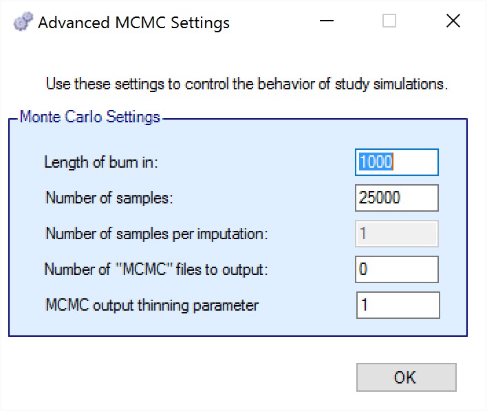
MCMC Settings
The first two values specify two standard MCMC parameters –
The length of burn-in is the number of the initial iterations whose results are discarded, to allow the sampled values to settle down.
The number of samples is the number of subsequent iterations whose results are recorded in order to give posterior estimates of the values of interest (in this case α and β).
Number of samples per imputation (not used in 2D-CRM, the model does not include imputation)
If the Number of MCMC samples to output value is set to N, where N > 0, then all the sampled values at each interim in the first N simulations are output in a file per simulation, allowing the user to check convergence.
The MCMC output thinning parameter can be used to reduce the amount of data output to the MCMC file. It does not reduce the amount of MCMC samples used within the model fitting.
To obtain the MCMC sampled values for a particular simulation, keep the same Random number seed and use Start at simulation to specify the simulation in question and run just 1 simulation.
How many simulations to run?
After first entering a design it is worth running just a small number of simulations such as 10 to check that the scenarios and design have been entered correctly. If all 10 simulations of a ‘null’ scenario are successful, or all 10 simulations of what was intended to be an effective drug scenario are futile, it is likely there has been a mistake or misunderstanding in the specification of the scenarios or the final evaluation or early stopping criteria.
Once the design and scenarios look broadly correct, it is usually worth quickly collecting rough estimates of the operating characteristics using around 100 simulations for each scenario. 100 simulations is enough to spot designs having very poor operating characteristics such as very high type-1 error, very poor power, a strong tendency to stop early for the wrong reason, or poor probability of selecting the correct target. 100 simulations is also usually sufficient to spot problems with the data analysis such as poor model fits and significant bias in the posterior estimates.
Typically 1,000 simulations of each scenario of interest is required to get estimates of the operating characteristics precise enough to compare designs and tune the parameters. (Very roughly rates of 5% (such as type-1 error) can be estimated to about +/-1.5% and rates of around 80% (such as power) estimated +/- 2.5%)
Finally around 10,000 simulations of the scenarios of interest is required to give confidence in operating characteristics of a design and possibly to select between the final shortlisted designs (Approximately rates of 5% can be estimated to about +/-0.5% and rates of around 80% estimated +/- 1%).
There may be many operating characteristics need to be compared over a number of scenarios, such as expected sample size, type-1 error, power, probability of selecting a good dose as the target and quality of estimation of the dose-response.
However frequently these will be compared over a range of scenarios, it may not be necessary to run very large number of simulations for each scenario if a design shows a consistent advantage on the key operating characteristics over the majority of the scenarios.
Simulation results
In the main screen the summary results that are usually of principal interest are displayed, the results summarised by scenario.
Show other columns: Allows the user to open additional windows on the simulation results, the windows available are:
All: A window containing all the summary results columns
Highlights: a separate window with the results shown on the main tab
Allocation, Observed: summary results of the number of subjects allocated, the number allocated to each dose, the number of toxicities observed and the number of toxicities observed per dose
Fitted toxicity: summary results of the estimates of the model parameters and the dose-toxicity.
Pr(MTD) etc: summary results of the posterior probabilities of the properties of interest
Simulation Results: a window displaying the individual simulation results for each simulation of the currently selected scenario
View Graph: opens the FACTS built in graph utility displaying the results for the currently selected scenario. See Error! Reference source not found. below for a description of the graphs.
Aggregate: opens a control that allows the user create aggregated results files from all the scenarios. The user can select which scenarios to include, and whether the results should be pivoted by dose. The resulting files are stored in the simulation results folder.
Open in R: If aggregated files have been created then clicking this button on the simulations tab will open control that allows the user to select which aggregations to load into data frames as R is opened. Otherwise it will offer to open R using the files in the currently selected scenario.
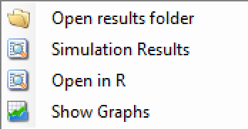
Right Click Menu: right clicking the mouse on a row of results in the simulation tab brings up a ‘local’ menu of options:
Open results folder: Opens a file browser in the results folder of the scenario, allowing swift access to any of the results files.
Simulation results: Opens a window displaying the individual simulation results for each simulation of the currently selected scenario
Open in R: opens a control that will launch R, first loading the selected files in the results folder as data frames.
Show Graphs: launches the graph viewer to view the results of the currently selected scenario.
FACTS Grid Simulation Settings
If you have access to a computational grid, you may choose to have your simulations run on the grid instead of running them locally. This frees your computer from the computationally intensive task of simulating so you can continue other work or even shutdown your PC or laptop. In order to run simulations on the grid, it must first be configured, this is normally done via a configuration file supplied with the FACTS installation by the IT group responsible for the FACTS installation.
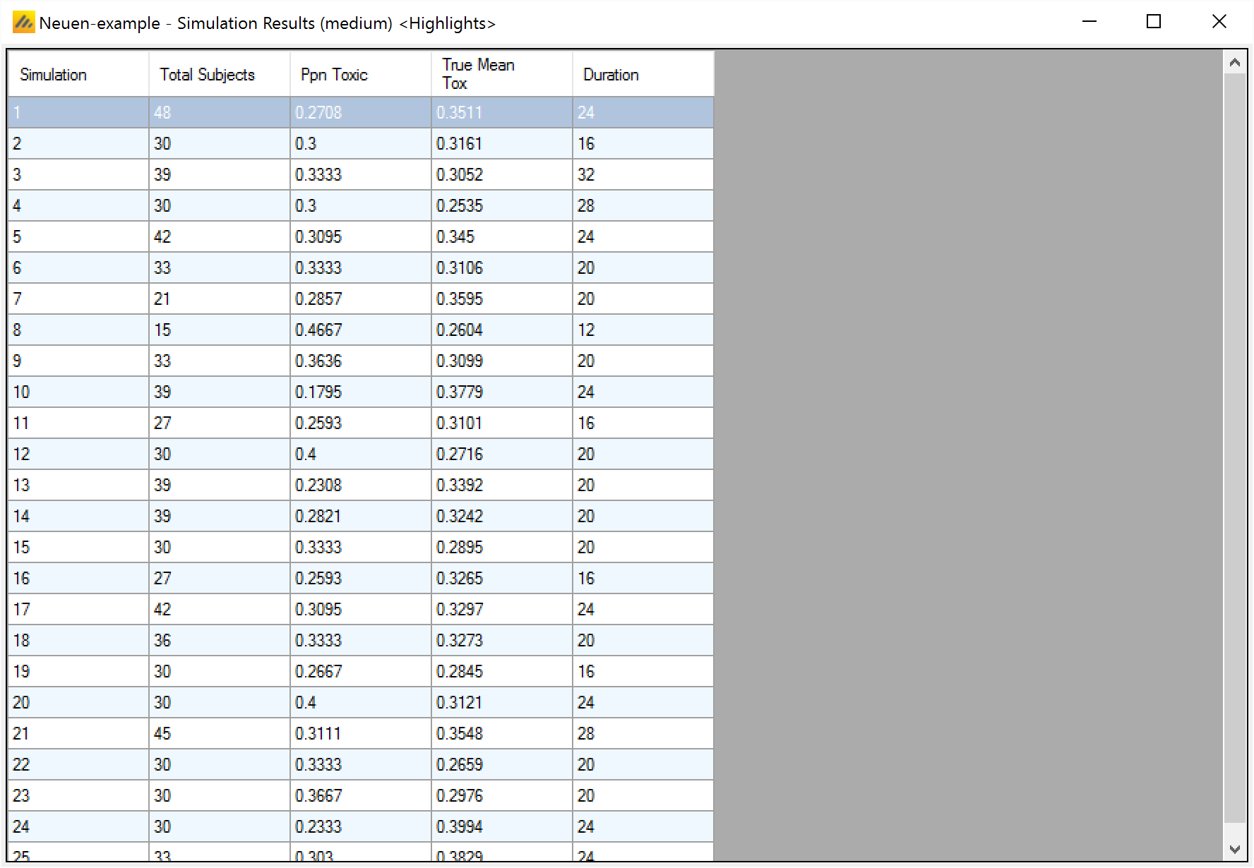
Detailed Simulation Results
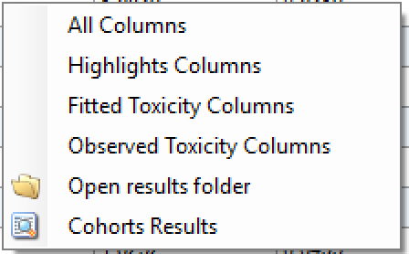
After simulation has completed and simulation results have been loaded, the user may examine detailed results for any scenario with simulation data in the table by double-clicking on the row. A separate window (as in Figure 17) shows the results simulation by simulation. Like the summary results – the initial window hold “highlights”, right clicking on the window displays a menu with options for viewing the “Fitted Toxicity”, “Observed Toxicity” or “All” Columns.
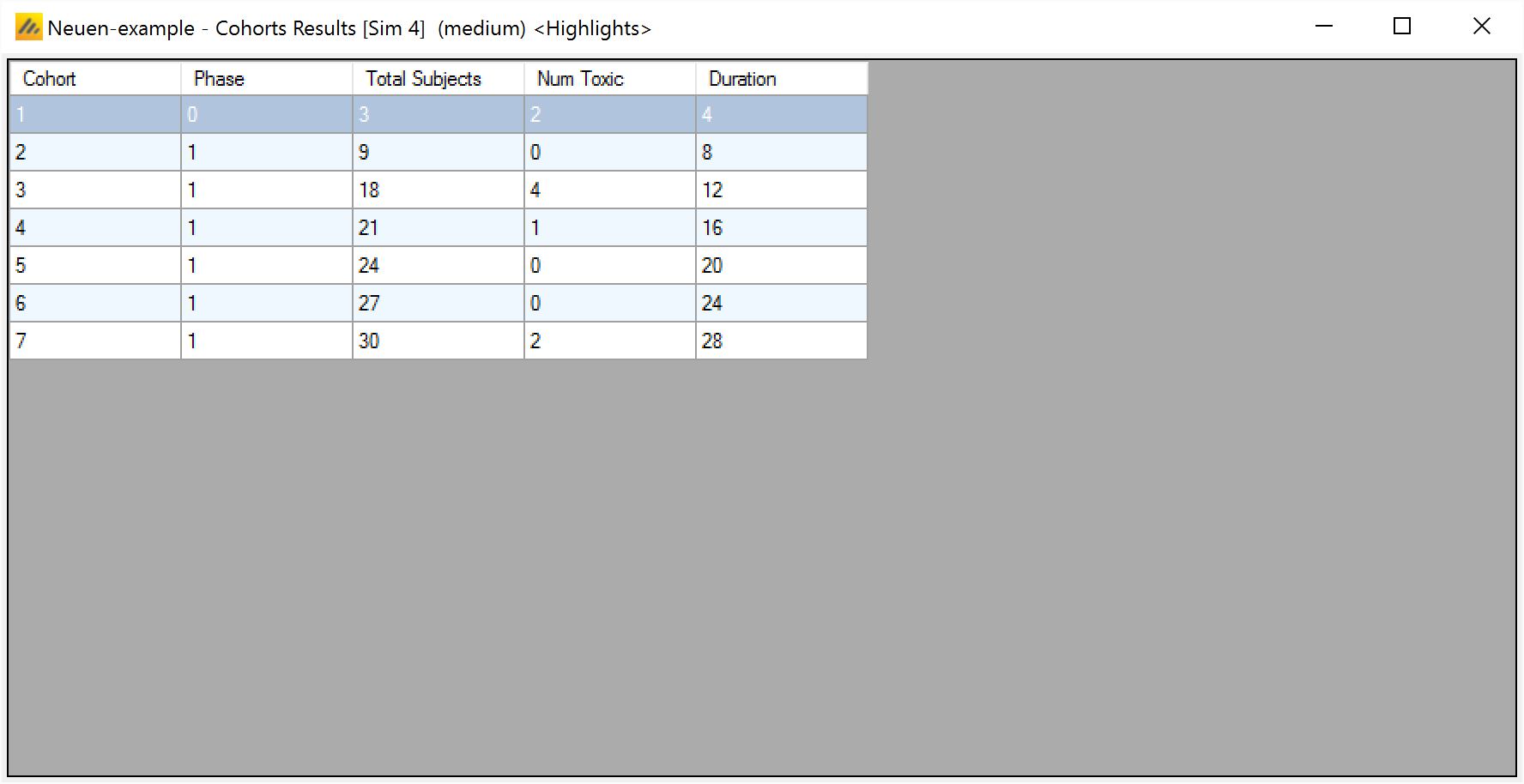
Cohort Simulation Results
After viewing individual simulation results, the user may examine detailed results for any simulation with per-cohort data in the table by right-clicking on the row and selecting “Cohort Results”. A separate window opens, showing the result for the selected simulation cohort by cohort. Like the summary and simulation results the initial window displays “highlights” columns, right clicking on the window displays a menu with options for viewing the “Fitted Toxicity”, “Observed Toxicity” or “All” Columns.
Aggregation
Aggregation combines the csv output from multiple scenarios into fewer csv files. The Aggregate… button displays a dialog which allows the user to select what to aggregate.
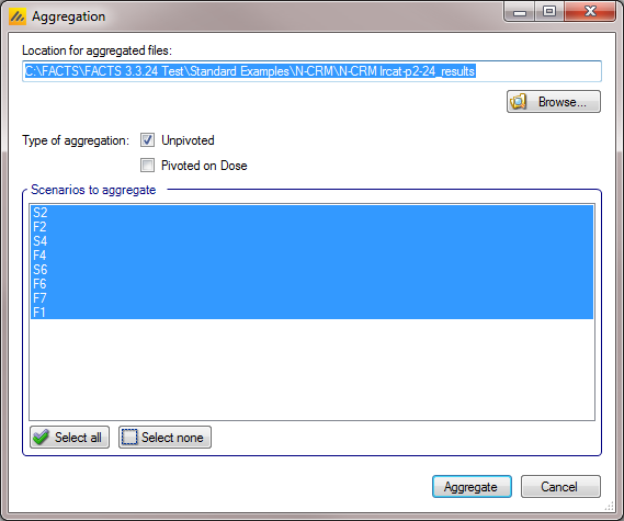
The default location for the aggregated files is the results directory for the study, but this can be changed.
In other design engines there is the option to pivot the results by dose, this is more complicated in 2D-CRM and the option is not available.
The default is to aggregate all scenarios, but any combination may be selected.
Pressing “Aggregate” generates the aggregated files.
Each type of csv file is aggregated into a separate csv file whose name begins agg_, so agg_summary.csv will contain the rows from each of the summary.csv files, cohortsNNN.csv files are aggregated into a single agg_cohorts.csv file. Doses.csv is identical for all scenarios and so is not aggregated.
Each aggregated file begins with the following extra columns, followed by the columns from the original csv file:
| Column Name | Comments |
|---|---|
| Scenario ID | Index of the scenario |
| Toxicity Profile | A series of columns containing the names of the various profiles used to construct the scenario. Columns that are never used are omitted (e.g External Subjects Profile if there are no external scenarios) |
| External Subjects Profile | |
| Agg Timestamp | Date and time when aggregation was performed |
| Sim | Simulation number. Only present in the cohorts file. |
| Dose | Only present if pivoted |
The Summary Results Columns
The simulation results are grouped into 4 tables; these tables can be opened by clicking the “Show Other Columns” button.
Highlights: these are the columns displayed in table on the Simulation tab.
Fitted Toxicity
Observed Toxicity
All – the combination of all the above.
The columns displayed in the first three tables are described in the subsections below.
Right clicking on any summary results table brings up a menu that allows the user to:
Open the results folder for the scenario line that the cursor is on
Open a window with the per simulation results
Open R and load the results as data frames
Open the FACTS graph display widow for the currently selected scenario.
Highlights
These are the columns displayed on the simulations tab after simulations are completed, the can also be displayed in the separate “Highlights” results window.
These results are in the ‘summar.csv’ files in each scenario results folder.
| Column Title | Number of columns | Description |
|---|---|---|
| Select | 1 | Not an output column, this column contains check box to allow the user to select which scenario to simulate. The ‘Select All’ button causes them all to be checked. |
| Status | 1 | This column reports on the current status of simulations: Completed, Running, No Results, Out of date, Error. It is updated automatically. |
| Scenario | 1 | This gives the name of the scenario. In the N-CRM this is simply the name of the Toxicity response profile to be simulated (in other Design Engines the scenario may be a combination of a number of profiles – e.g. one for the toxicity response and one for the efficacy response). |
| Num Sims | 1 | The number of simulations that are being summarised |
| Mean subjects | 1 | The mean number (over the simulations) of subjects randomized |
| Ppn Toxic | 1 | The mean (over the simulations) proportion of the randomized subjects that had a toxic outcome |
| Sd Ppn Toxic | 1 | The standard deviation (over the simulations) of the proportion of subjects that had a toxic outcome. |
| Mean true toxicity | 1 | The mean (over the simulations) of the true probabilities of toxicity that subjects have been exposed to. |
| Duration | 1 | The mean duration of the simulations in weeks |
| Sd Duration | 1 | The standard deviation of the durations of the simulations |
| Ppn All Toxic | 1 | The proportion of the simulations that stopped because all combinations were judged too toxic (exceeded the overdose control limit). |
| Ppn Early Succ | 1 | The proportion of the simulations that stopped because the stopping condition(s) had been satisfied. |
| Ppn Reached Cap | 1 | The proportion of the simulations that stopped because the maximum nmber of subjects had been reached. |
| Ppn MTT Under | 1 | The proportion of the dose combinations selected as MTT that actually had a toxicity rate in the “under-dosing” range. |
| Ppn MTT Target | 1 | The proportion of the dose combinations selected as MTT that actually had a toxicity rate in the “target” range. |
| Ppn MTT Excess | 1 | The proportion of the dose combinations selected as MTT that actually had a toxicity rate in the “excess” range. |
| Ppn MTT Unacceptable | 1 | The proportion of the dose combinations selected as MTT that actually had a toxicity rate in the “unacceptable” range. |
| Ppn Correct Under | 1 | The proportion of the dose combinations that have a true toxicity rate in the “under-dosing” band over all the simulations that are determined to be “under-dosing”. That is the posterior probability at the end of the simulation that the toxicity rate of that dose combination of being in the “under-dosing” band is greater than the probabilities of being in the “target” band or the combined “excess” and “unacceptable” toxicity bands, and the combination is not excluded by the overdose control conditions. |
| Ppn Correct Target | 1 | The proportion of the dose combinations that have a true toxicity rate in the “target” band over all the simulations that are determined to be “target”. That is the posterior probability at the end of the simulation that the toxicity rate of that dose combination of being in the “target” band is greater than the probabilities of being in the “under-dosing” band or the combined “excess” and “unacceptable” toxicity bands, and the combination is not excluded by the overdose control conditions. |
| Ppn Excess+Unacc | 1 | The proportion of the dose combinations that have a true toxicity rate in the “excess” or “unacceptable” bands over all the simulations that are determined to be “excess” or “unacceptable”. That is the posterior probability at the end of the simulation that the toxicity rate of that dose combination of being in the “excess” or “unacceptable” bands is greater than the probabilities of being in the “under-dosing” band or the “target band”, or the combination is excluded by the overdose control conditions. |
Fitted Toxicity
| Column Title | Number of columns | Description |
|---|---|---|
| Status | 1 | This column reports on the current status of simulations: Completed, Running, No Results, Out of date, Error. It is updated automatically. |
| Scenario | 1 | This gives the name of the scenario. In the N-CRM this is simply the name of the Toxicity response profile to be simulated (in other Design Engines the scenario may be a combination of a number of profiles – e.g. one for the toxicity response and one for the efficacy response). |
| Mean Tox Coeffs | 5 | The mean (over the simulations) of the estimate of the 5 parameters of the BLRM Dose-Toxicity model |
| Sd Tox Coeffs | 5 | The standard deviation (over the simulations) of the estimate of the 5 parameters of the BLRM Dose-Toxicity model |
| Pr(Under): <Dose>, <Dose> | I*J | The mean (over the simulations) of the posterior probability of being under the target toxicity at each dose combination. |
| Pr(Target): <Dose>, <Dose> | I*J | The mean (over the simulations) of the posterior probability of being in the target toxicity band at each dose combination |
| Pr(Excess): <Dose>, <Dose> | I*J | The mean (over the simulations) of the posterior probability of being in the excess toxicity band at each dose combination |
| Pr(Unacc): <Dose>, <Dose> | I*J | The mean (over the simulation) of the posterior probability of being in the unacceptable toxicity band at each dose combination |
| Pr(Sel-MTT): <Dose>, <Dose> | I*J | The proportion of times that each dose combination was selected as the combination with the MTT (Maximum Target Toxicity). Some methods may select more than one such combination so that these proportions sum to more than one for each scenario. |
| Mean Fitted Tox: <Dose>, <Dose> | I*J | The mean (over the simulations) of the estimate of the toxicity rate at each dose combination. |
| Sd Fitted Tox: <Dose>, <Dose> | I*J | The standard deviation (over the simulations) of the toxicity rate at each dose combination. |
Observed Toxicity
| Column Title | Number of columns | Description |
|---|---|---|
| Status | 1 | This column reports on the current status of simulations: Completed, Running, No Results, Out of date, Error. It is updated automatically. |
| Scenario | 1 | This gives the name of the scenario. In the N-CRM this is simply the name of the Toxicity response profile to be simulated (in other Design Engines the scenario may be a combination of a number of profiles – e.g. one for the toxicity response and one for the efficacy response). |
| Mean Subjects: <Dose>, <Dose> | I*J | The mean (over the simulations) of the number of subjects allocated to each dose combination. |
| Sd Subjects: <Dose>, <Dose> | I*J | The standard deviation (over the simulations) of the number of subjects allocated to each dose combination. |
| Mean Obs Tox: <Dose>, <Dose> | I*J | The mean (over the simulations) of the number of observed toxicities at each dose combination. |
| Sd Obs Tox: <Dose>, <Dose> | I*J | The standard deviation (over the simulations) of the number of observed toxicities at each dose combination. |
The Per-Simulation Results
Double clicking on any row in the simulation results table, opens a window displaying the individual simulation results. This table shows the individual results that are averaged in the summary table.
These values are in the ‘simulations.csv’ for each scenario in the scenario results folder.
Like the summary results, the per-simulation results are organized into ‘Highlights’, ‘Fitted Toxicity’ and ‘Observed Toxicity’ tables, with the corresponding columns.
Right clicking on any summary results table brings up a menu that allows the user to:
Open the per-simulations results window with all columns
Open the per-simulations results window with the highlights columns
Open the per-simulations results window with the fitted toxicity columns
Open the per-simulations results window with the observed toxicity columns
Open the results folder for the scenario line that the cursor is on
Open the cohort results widow for the currently selected simulation.
Graphs
There are 7 “overall” graphs that show means over the simulations and 5 graphs that show results per simulation or per cohort per simulation and one graph that shows the “true” toxicity – that is the toxicity rates being simulated for each dose combination in the scenario. The per cohort graphs can only be displayed for those simulations with “full results” (the number of these is specified on the “Advanced” dialog window on the Simulations tab), that is a “cohortsNNNN.csv” file has been written out for that simulation (where “NNNN” is replaced by the simulation number).
The 7 Overall graphs are:
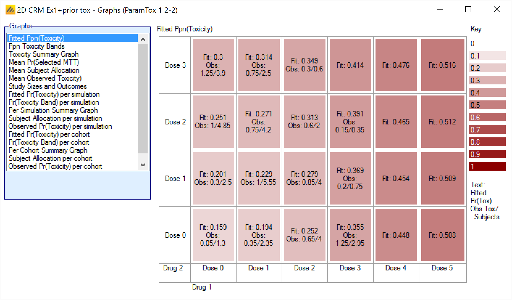
Fitted Ppn(Toxicity) – Displays the mean of the fitted mean toxicity rates at each dose combination, the cells are colored according to the fitted rate, also shows the mean observed number of toxicities and mean number of subjects exposed at each dose combination.
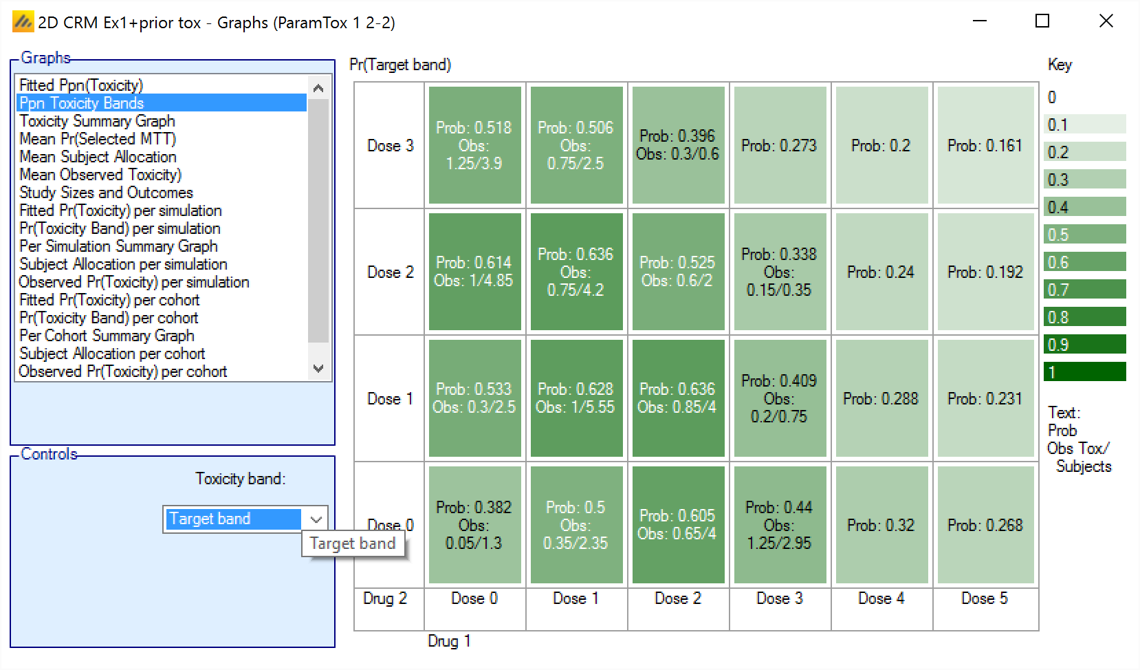
Ppn Toxicity Bands – Displays the mean of the posterior probabilities that the toxicity rate lies in the selected toxicity band at each dose combination, also shows the mean observed number of toxicities and mean number of subjects exposed at each dose combination.
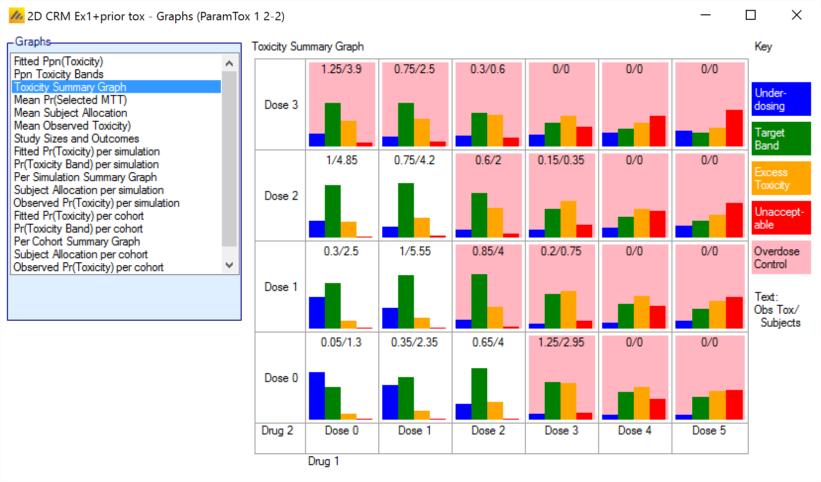
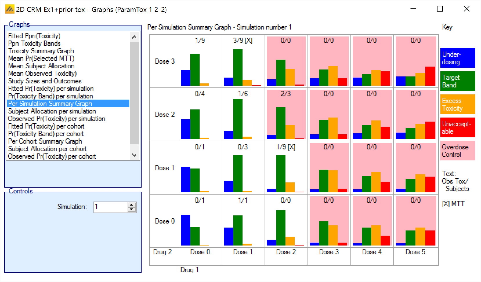
Toxicity Summary Graph – Displays a small histogram for each dose combination, plotting the mean probability that the toxicity rate lies in each of the toxicity bands, also highlights those dose combinations that would be exclude based on applying the overdose control rules to the mean probabilities.
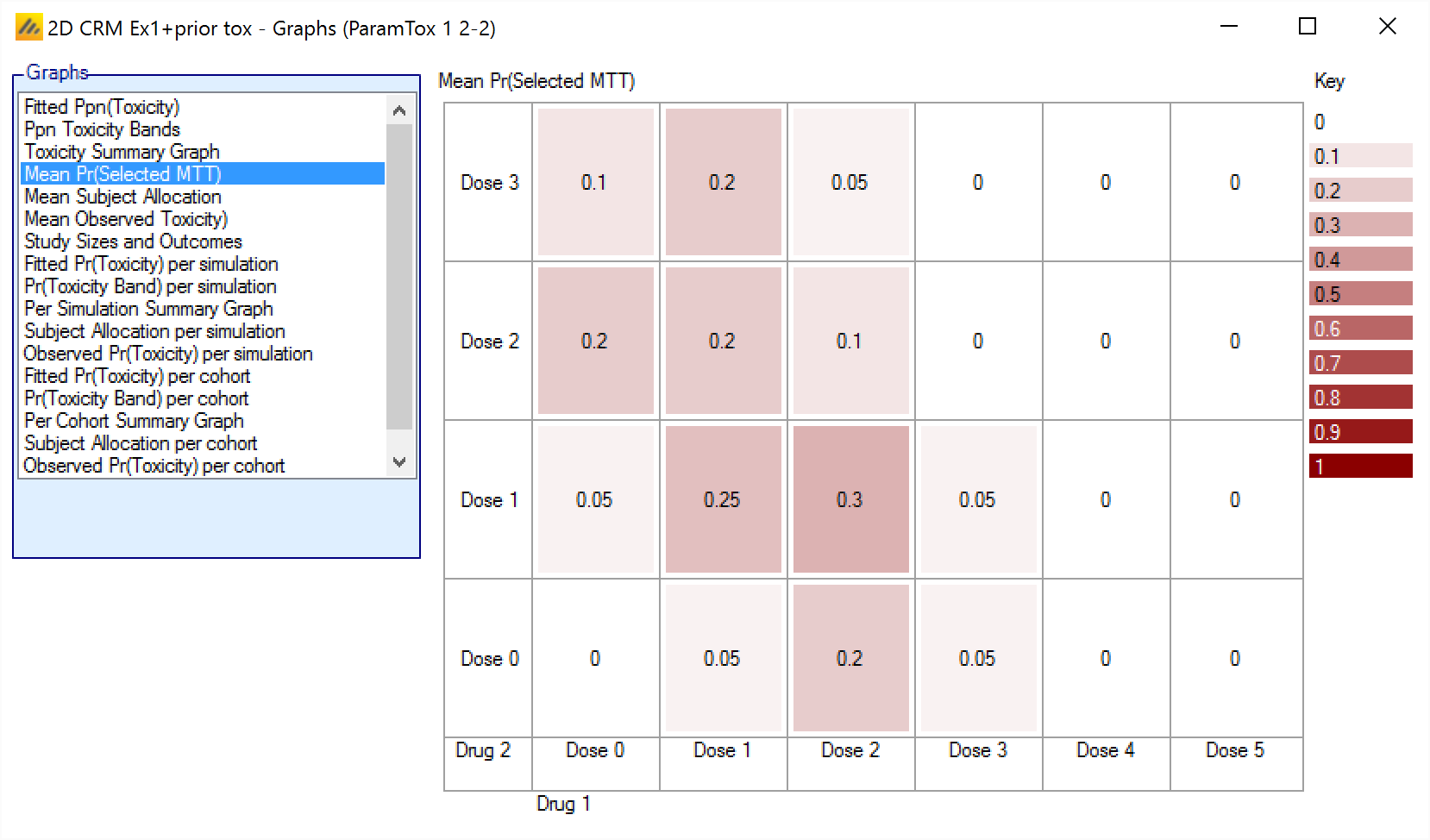
Mean Pr(Selected MTT) – Displays the ppn of times each dose combination was selected as MTT (Maximum probability of being in the Target Toxicity band) (depending on the Dose Escalation method employed, there may be more than one combination selected as MTT at the end of each simulation).
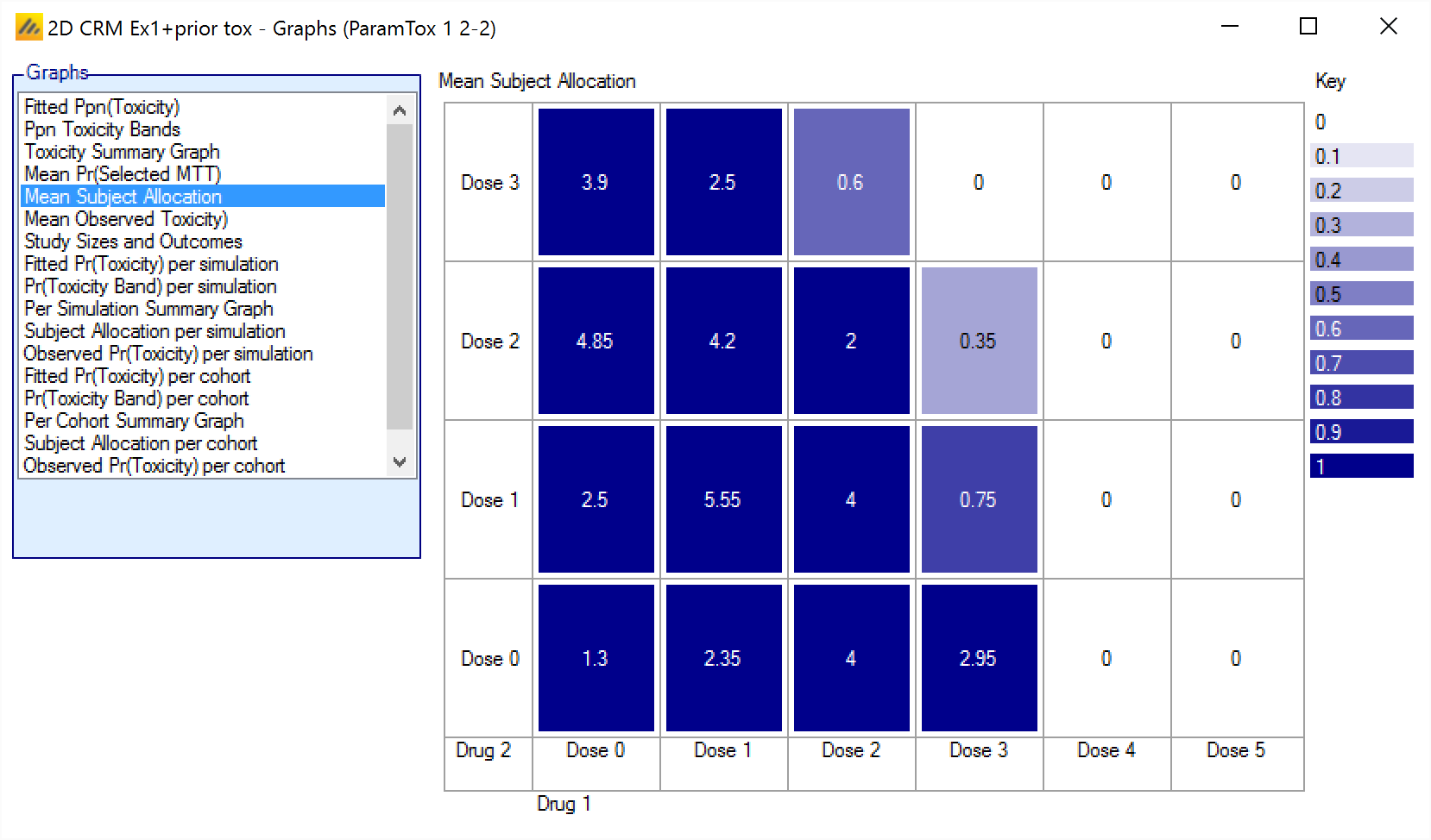
Mean Subject Allocation – Displays the mean number of subjects allocated to each dose combination.
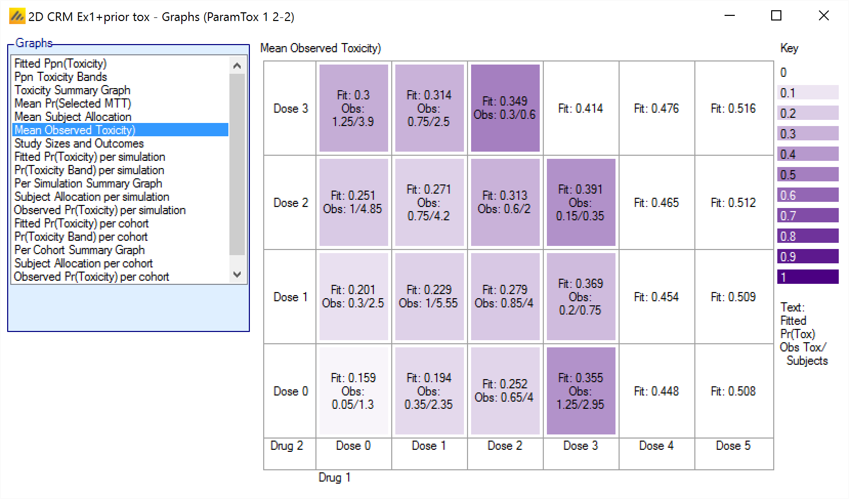
Mean Observed Toxicity – Displays the mean of the fitted mean toxicity rates at each dose combination, also shows the mean observed number of toxicities and mean number of subjects exposed at each dose combination. The cells are colored according to the observed toxicity ratio.
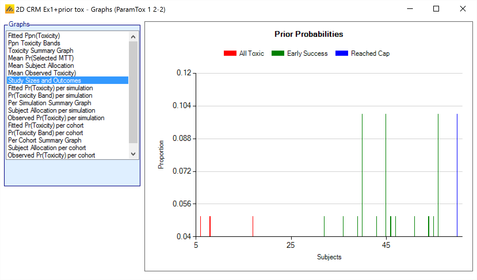
Study Sizes and Outcomes – Displays a histogram of the Ppn of simulations that completed at different sample sizes, colored to indicate their reason for stopping.
The 5 per-simulation and per-cohort graphs are
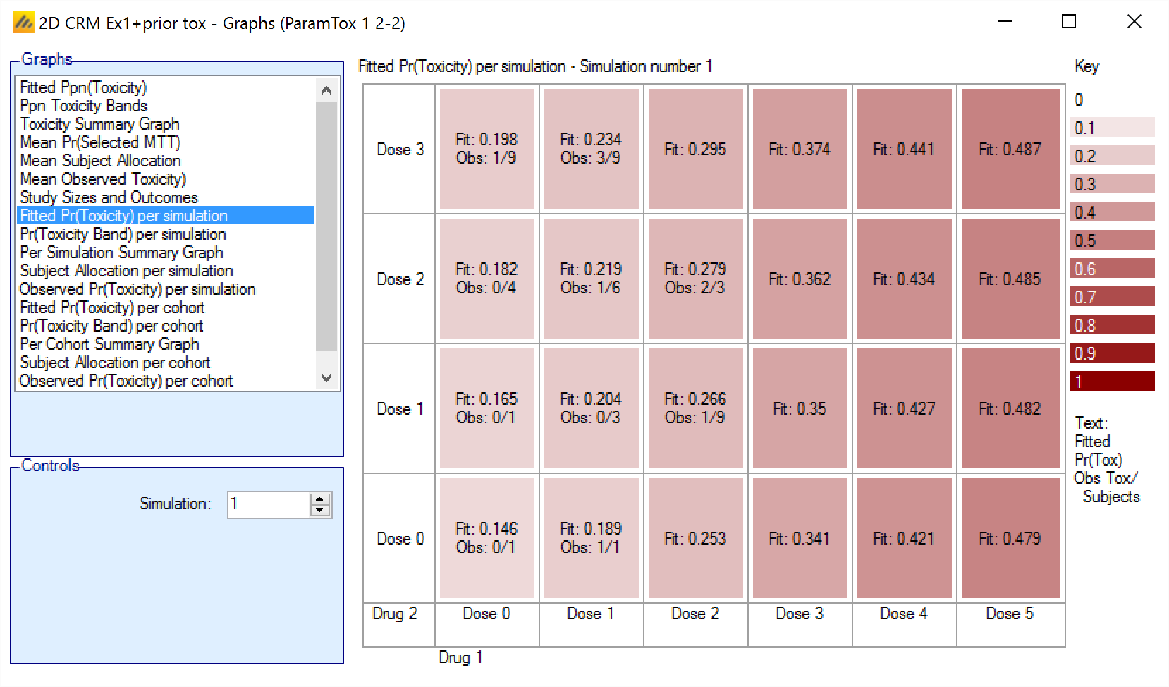
Fitted Pr(Toxicity) – Displays fitted mean toxicity rate at each dose combination, the cells are colored according to the fitted rate, also shows the observed number of toxicities and the number of subjects exposed at each dose combination.
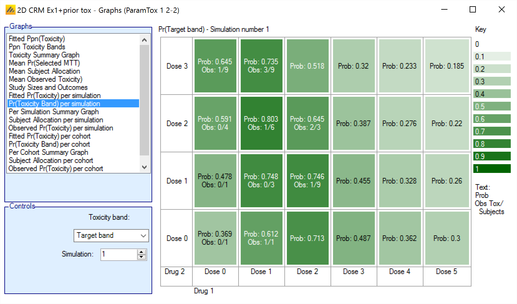
Pr(Toxicity Band) - Displays the posterior probability that the toxicity rate lies in the selected toxicity band at each dose combination, also shows the observed number of toxicities and number of subjects exposed at each dose combination.
Summary graph - Displays a small histogram for each dose combination, plotting the probability that the toxicity rate lies in each of the toxicity bands, also highlights those dose combinations that are excluded based on applying the overdose control rules to the probabilities.
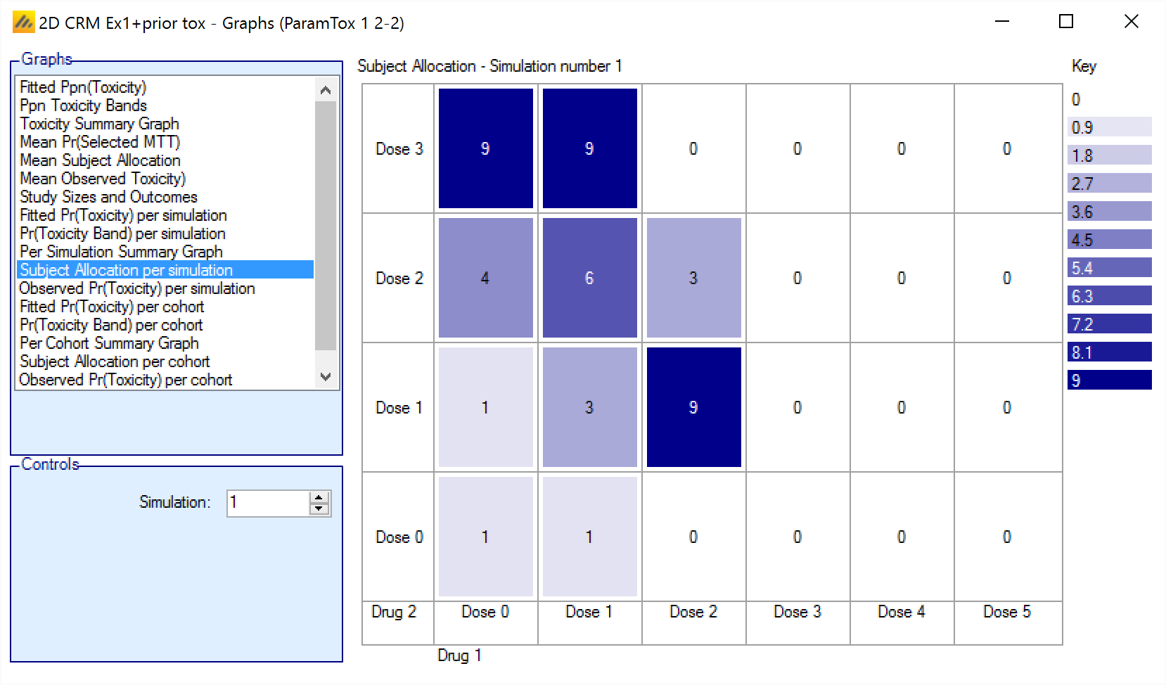
Subject Allocation - Displays the number of subjects allocated to each dose combination.
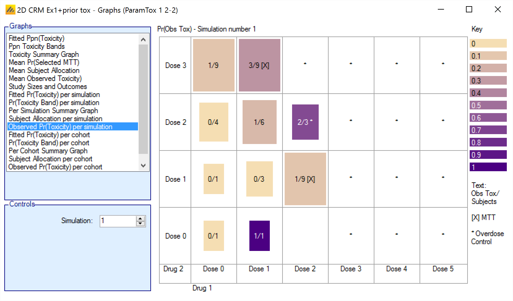
Observed Pr(Toxicity) - Displays the fitted mean toxicity rate at each dose combination, also shows the observed number of toxicities and the number of subjects exposed at each dose combination. The cells are colored according to the observed toxicity ratio. The dose combinations selected as MTT / next combinations to allocate to are indicated.
Fitted Ppn(Toxicity)
The Fitted Ppn(Toxicity) graph shows the average mean posterior estimate of the toxicity at each combination, with the cells colored in increasing intensity the higher the fitted toxicity. In addition in each cell the average number of observed toxicities and average total observations is reported.
The format is:
Fit: <Average Mean estimate of toxicity>
Obs: <Mean toxicity observations> / <Mean total observations>
Ppn(Toxicity Bands)
The Ppn(Toxicity Bands) graph shows the average mean posterior estimate that the toxicity falls in one of the defined toxicity bands, with the cells colored from faint to intense the higher the probability. The color used depends on the band being displayed: blue for under-dosing, green for target, orange for excess and red for unacceptable.
In addition in each cell the average number of observed toxicities and average total observations is reported.
The format is:
Prob: <Average Posterior Probability>
Obs: <Mean toxicity observations> / <Mean total observations>
Toxicity Summary Graph
The Toxicity Summary Graph displays a small histogram for each dose combination. In each histogram it shows for that dose combination the posterior probability its toxicity rate is in each of the four toxicity bands.
If the posterior probabilities are such that the dose combination is excluded by the overdose control rules, then the background of the histogram is in pink to highlight it.
Mean Pr(Selected MTT)
The Mean Pr(Selected MTT) graph shows the average number of times each combination was selected as the, or one of the, combinations with Maximum Target Toxicity. The cells are colored more intensely the greater the Ppn of simulations that the dose combination was selected as MTT.
The ‘Selected as MTT’ dose combination is the one with the maximum posterior probability of having a toxicity rate in the target band and not excluded by overdose control. The ‘Walk’ and ‘Allocate to MTT’ dose escalation methods select a single MTT at the end of a trial, but the ‘Contour’ and ‘Tri-Axial’ can select multiple MTTs so when using these dose escalation methods these probabilities can sum to more than 1.
The format is:
<PPn of simulations this combination selected as MTT>
Mean Subject Allocation
The Mean Subject Allocation graph shows the average number of subjects allocated to each combination over all the simulations, with the cells colored from white to dark blue the greater the number allocated.
The format is:
<Number of subjects allocated to this combination>
Mean Observed Pr(Toxicity)
The Mean Observed Pr(Toxicity) graph shows the average number of observations and number of toxicities along with the mean fitted toxicity across all the simulations. The color intensity reflects the fraction of observations that resulted in toxicity, with the color more intense the closer that fraction gets to 1..
The format is:
Fit: <Average Mean Estimate of Toxicity>
Obs: <Mean toxicity observations> / <Mean total observations>
Study Sizes and Outcomes
The Study Sizes and Outcomes graph plots a histogram, of the sample sizes of the simulations. The bars are colored to show why the simulated trial stopped:
Because all dose combinations were too toxic (barred by the overdose control rules)
Because defined stopping rule had been met.
Because the trial maximum sample size had been reached.
Fitted Pr(Toxicity) per simulation/per cohort
The Fitted Ppn(Toxicity) graph shows the mean posterior estimate of the toxicity at each combination for each simulation, with the cells colored from beige to intense red the higher the toxicity. In addition in each cell the number of observed toxicities and total observations is reported.
For simulations for which a “cohortNNNN.csv” file was output, the graph can be viewed for the result of the analysis after each cohort – allowing the trial to be “stepped through” a cohort at a time.
The format is:
Fit: <Mean estimate of toxicity>
Obs: < Toxicity observations> / <Total observations>
Pr(Toxicity Band) per simulation/per cohort
The Ppn(Toxicity Bands) graph shows the posterior estimate that the toxicity falls in one of the defined toxicity bands for each simulation, with the cells colored from faint to intense the higher the probability. The color used depends on the band being displayed: blue for under-dosing, green for target, orange for excess and red for unacceptable.
In addition in each cell the number of observed toxicities and total observations is reported.
For simulations for which a “cohortNNNN.csv” file was output, the graph can also be viewed for the result of the analysis after each cohort – allowing the trial to be “stepped through” a cohort at a time.
The format is:
Prob: <The Posterior Probability>
Obs: <The number toxicity observations> / <The number of total observations>
Summary Graph per simulation/per cohort
The Summary graph shows the posterior estimate that the toxicity falls into each of the defined toxicity bands as a small histogram for each dose combination
In addition in the cells where the dose combination is excluded by the overdose rules are highlighted with a pink background.
Subject Allocation per simulation/per cohort
The Subject Allocation graph shows the number of subjects allocated to each combination in a particular simulation with the cells colored from white to dark blue the greater the number allocated.
For simulations for which a “cohortNNNN.csv” file was output, the graph can also be viewed for the subject allocation after each cohort – allowing the trial to be “stepped through” a cohort at a time.
The format is:
<Number of subjects allocated to this combination>
Observed Pr(Toxicity) per simulation/per cohort
The Observed Pr(Toxicity) graph shows the number of observations and number of toxicities for each combination, for each the simulation. The color intensity reflects the fraction of observations that resulted in toxicity, with the color more intense the closer that fraction gets to 1.The size of the colored square is proportional to the number of observations.
For simulations for which a “cohortNNNN.csv” file was output, the graph can also be viewed for the subject allocation after each cohort – allowing the trial to be “stepped through” a cohort at a time.
The format is:
Obs: <Mean toxicity observations> / <Mean total observations>
Cells excluded by the overdose control rules are marked with a “*”.
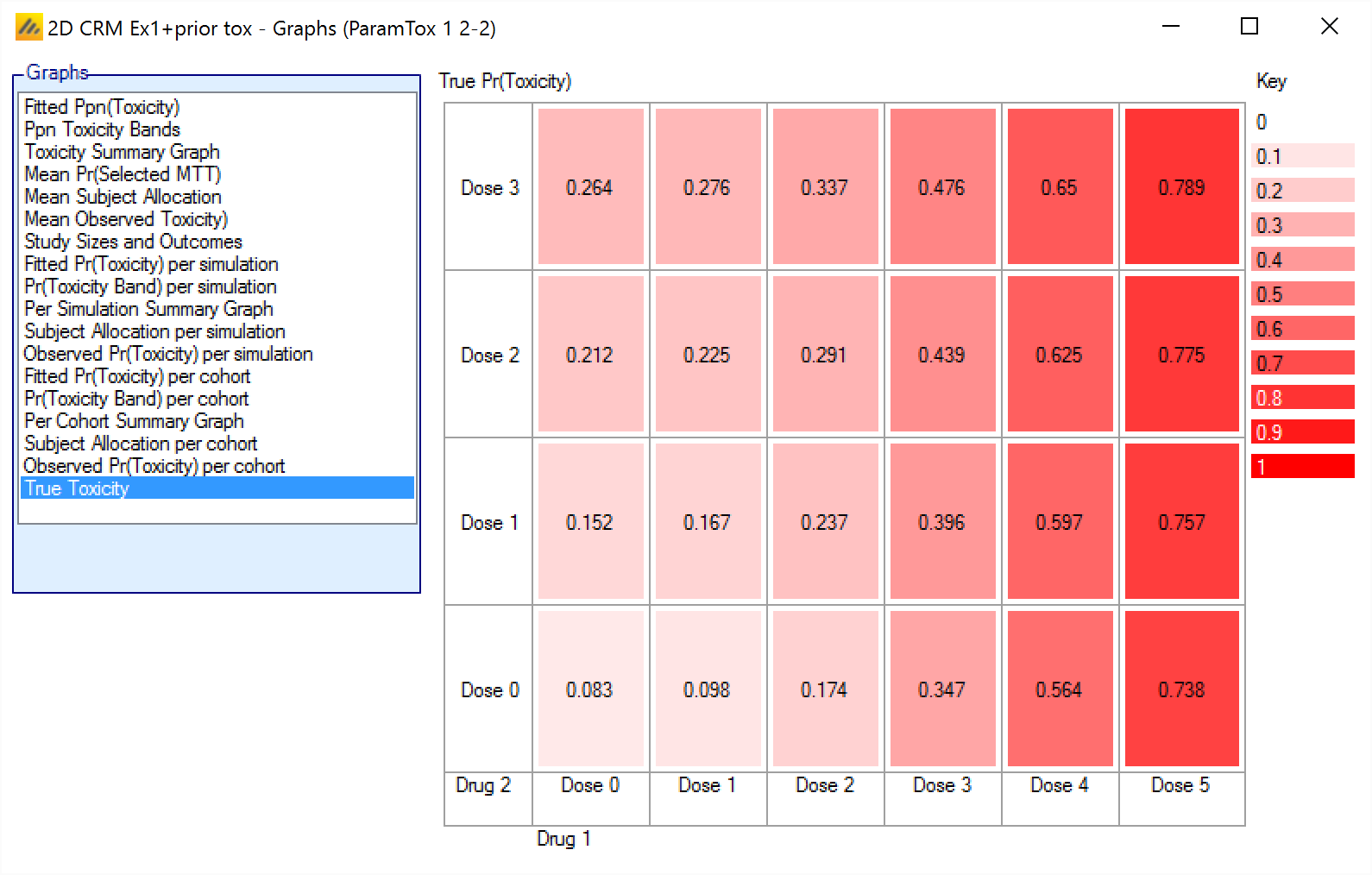
True Pr(Toxicity)
The True Ppn(Toxicity) graph shows the toxicity rate simulated at each combination for all the simulations, with the cells colored from beige to intense red the higher the toxicity.
The format is:
<Simulated toxicity rate>
Analysis Tab
Initially the Analysis tab just displays a “Use Design to Analyze Data” button.
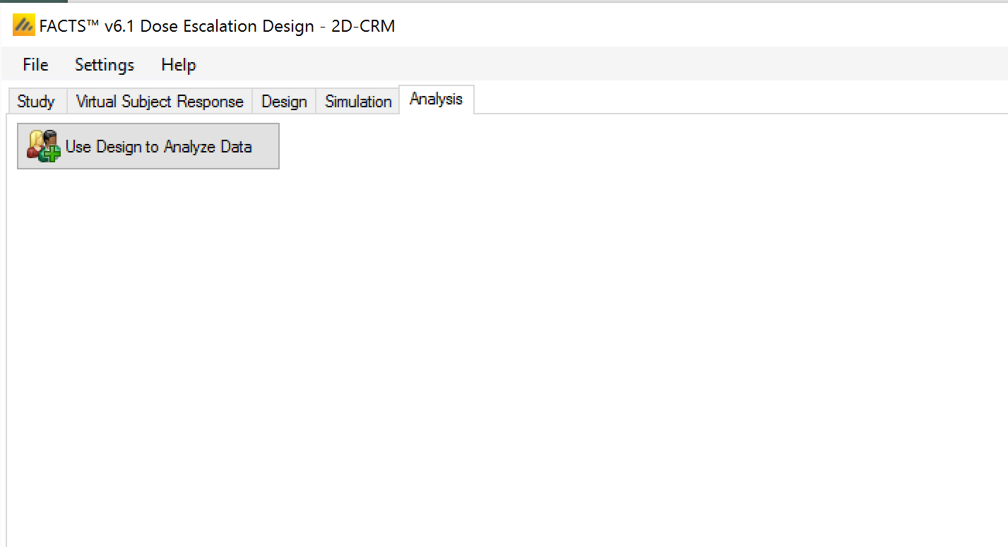
After clicking the button the tab becomes active,
and an “Analysis” folder is created alongside the folder that hold the simulation results.
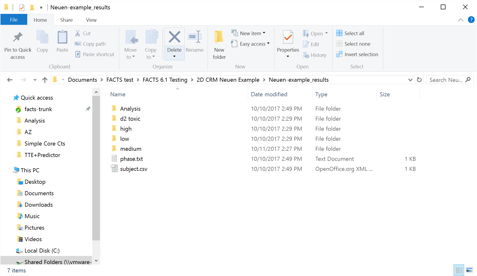
In the “…_Results” folder there an empty “subject.csv file will have been created
This is the file that should be edited to contain the data to be analyzed, or the data can be added via the FACTS User Interface through the Analysis > Subject Data tab.
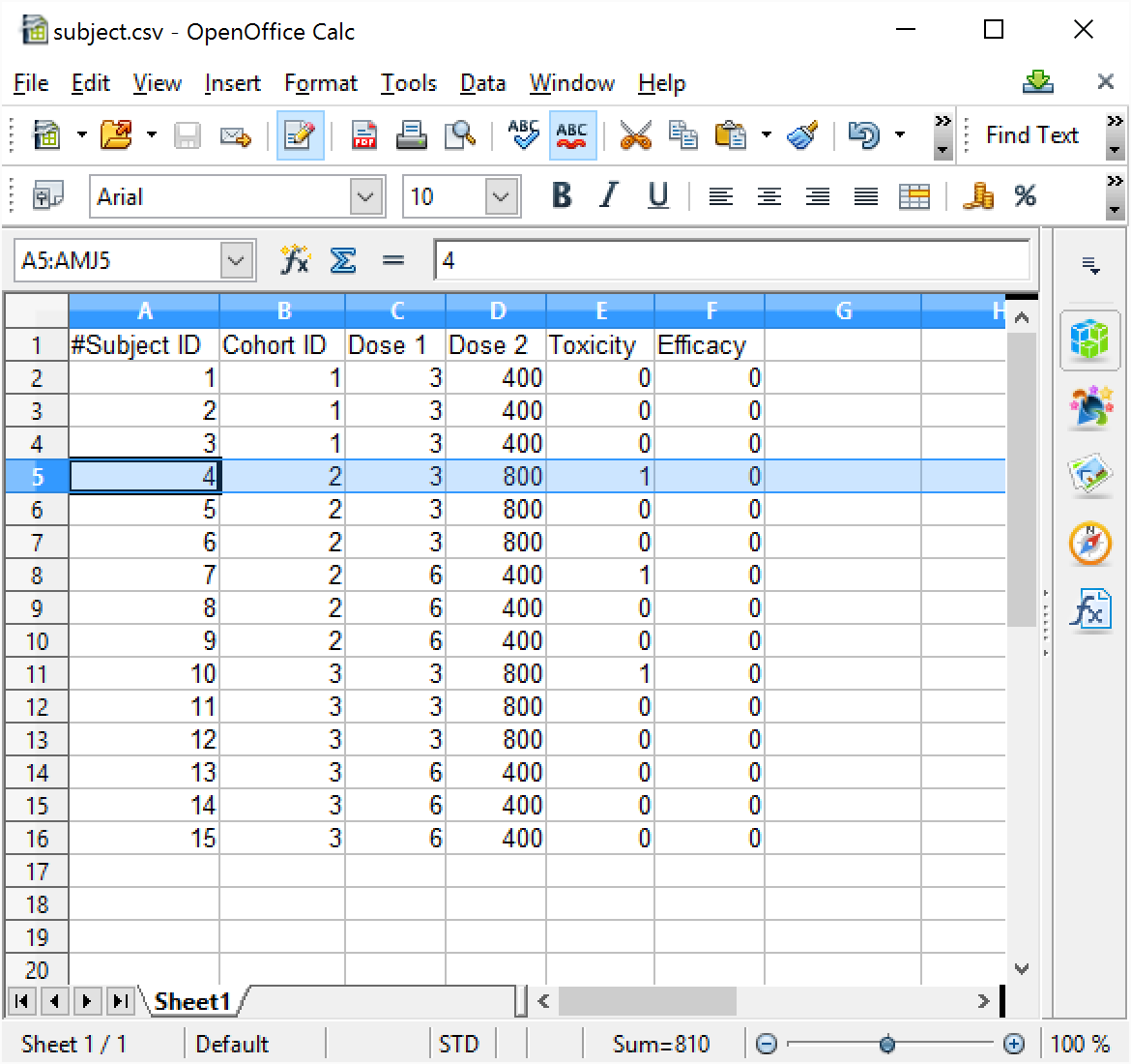
The file format is a comma separated text file. The file must contain the following fields/columns:
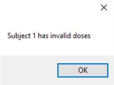
- Subject ID: the id of the subject. This should simply be a numeric value. It is unused by the 2D-CRM engine, it is provided as an aid to linking the record to actual patient data (if that is what is being used). It is useful to give each subject a different Id as errors in the file are reported by 2D-CRM using the Subject ID Num:
Cohort ID: the number of the cohort the subject was treated in. This should be a simple increasing integer, but of course several subjects will belong to the same cohort.
Dose 1, Dose 2: these should be the strength of the dose of Drug 1 and Drug 2 that the subject was treated with, doses are indexed 1, 2, 3, …. Max dose.
Toxicity: this value indicates whether the subject had a dose limiting toxicity or not. It should be 0 (to indicate no toxicity) or 1 (to indicated toxicity).
Efficacy: This value is included for future expansion to additionally taking an efficacy response into account. It should be 0 or 1. The value is currently ignored.
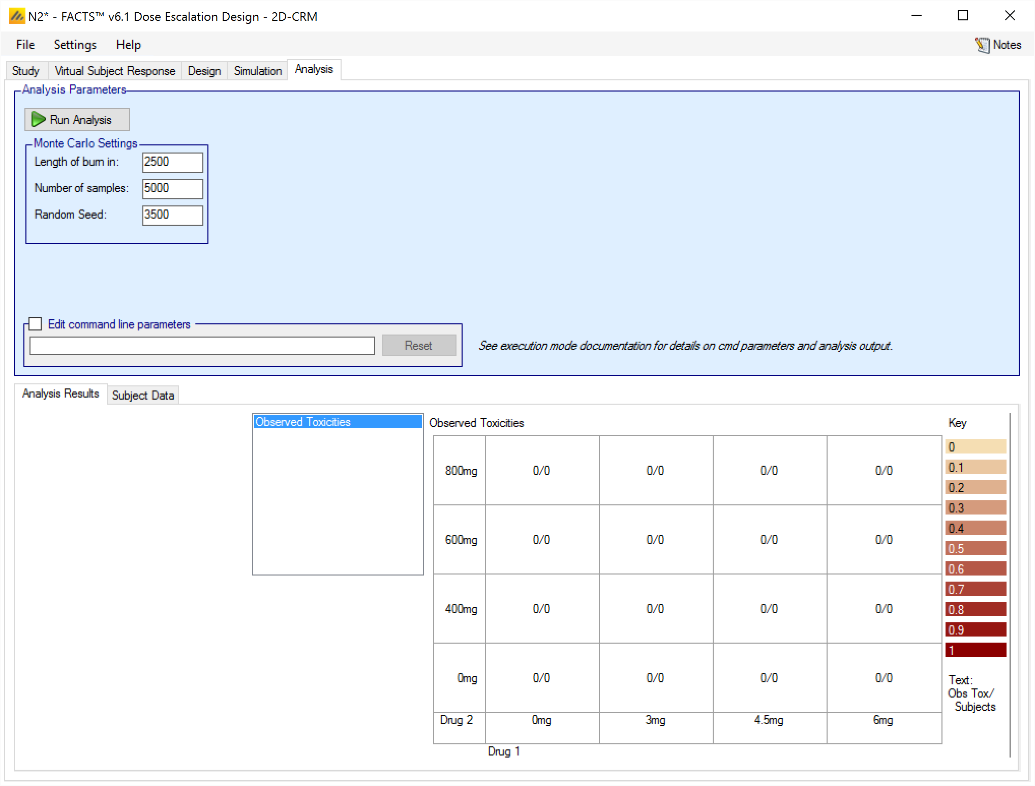
After entering the above into the subjects.csv and then clicking on “Reload Data”, the Analysis tab looks like this:
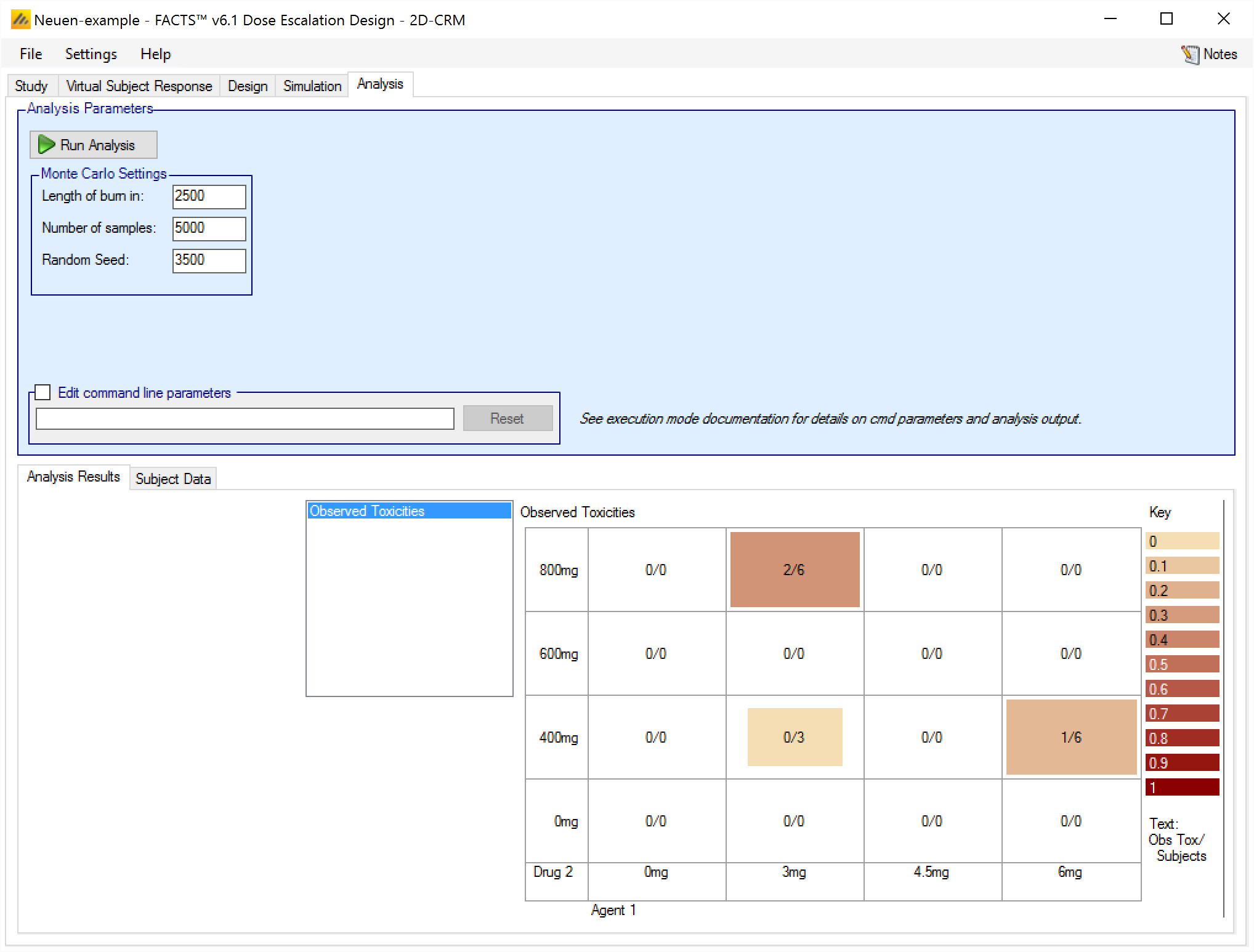
We can see that the data has been correctly loaded – 4 subjects with no toxicity on combination (3mg,400mg), 6 subjects with 2 toxicity on combination (3mg,800mg) and 6 subjects with 1 toxicity on combination (6mg,400mg). But as yet no analysis has been run. To run an analysis on this data, click on “Run Analysis”.
Once the analysis has completed, the screen looks like this …
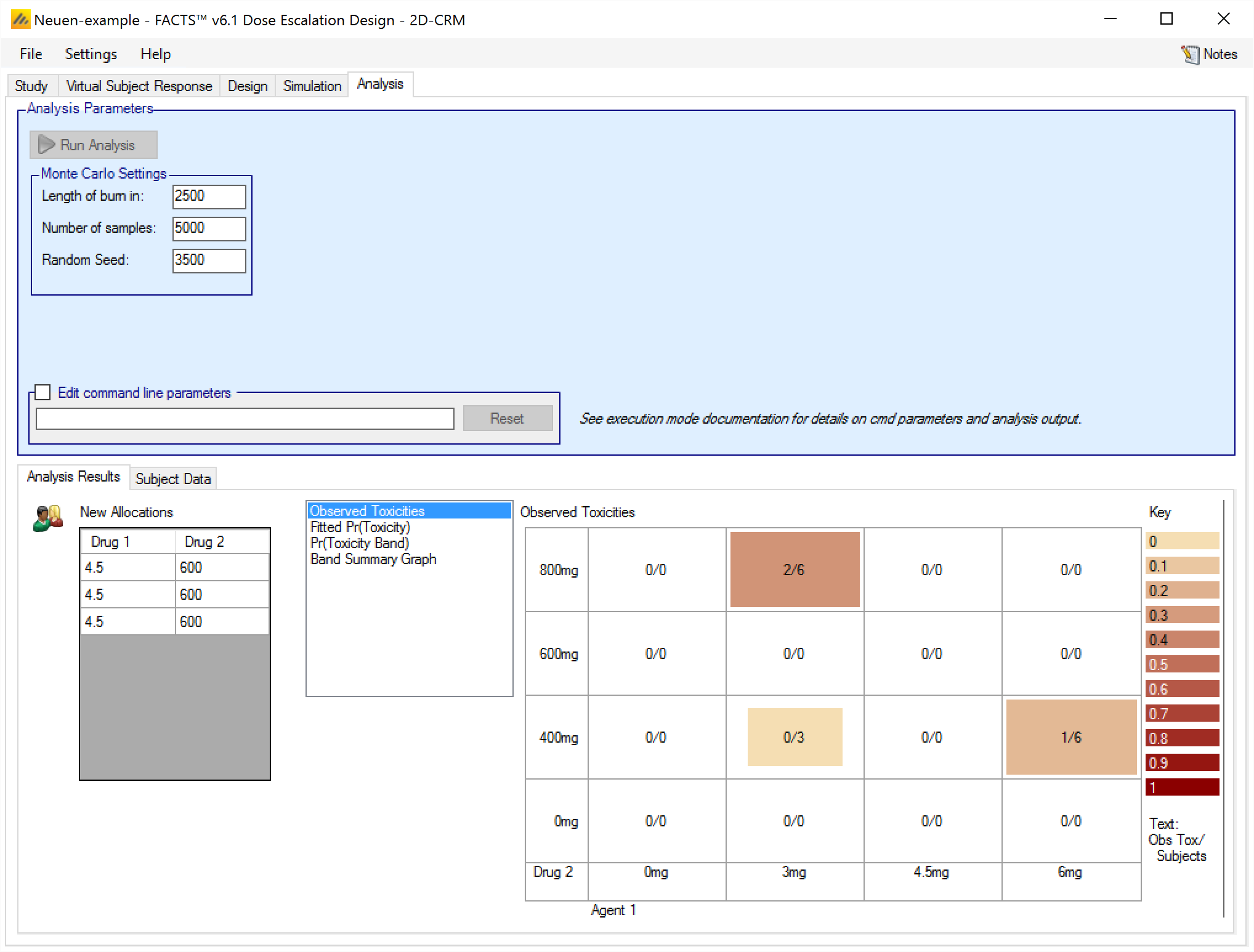
We can see that the next recommended combinations are (4.5mg,600mg)
In the simulation of the design that has been entered, all the combinations recommended would be tested by allocating a cohort to each combination in the next round. In practice the clinical team would review these recommendations, the results of the model fit and possibly other data such as minor toxicities observed to form a view as to which combinations should be tested.
Analysis tab graphs
After the analysis the graph shown by default is the “Observed Toxicities” graphs (shown above).
The other three graphs available are similar to the “per cohort” graphs available for simulations, namely:
Fitted Pr(Toxicity)
Pr(Toxicity band)
Band Summary Graph
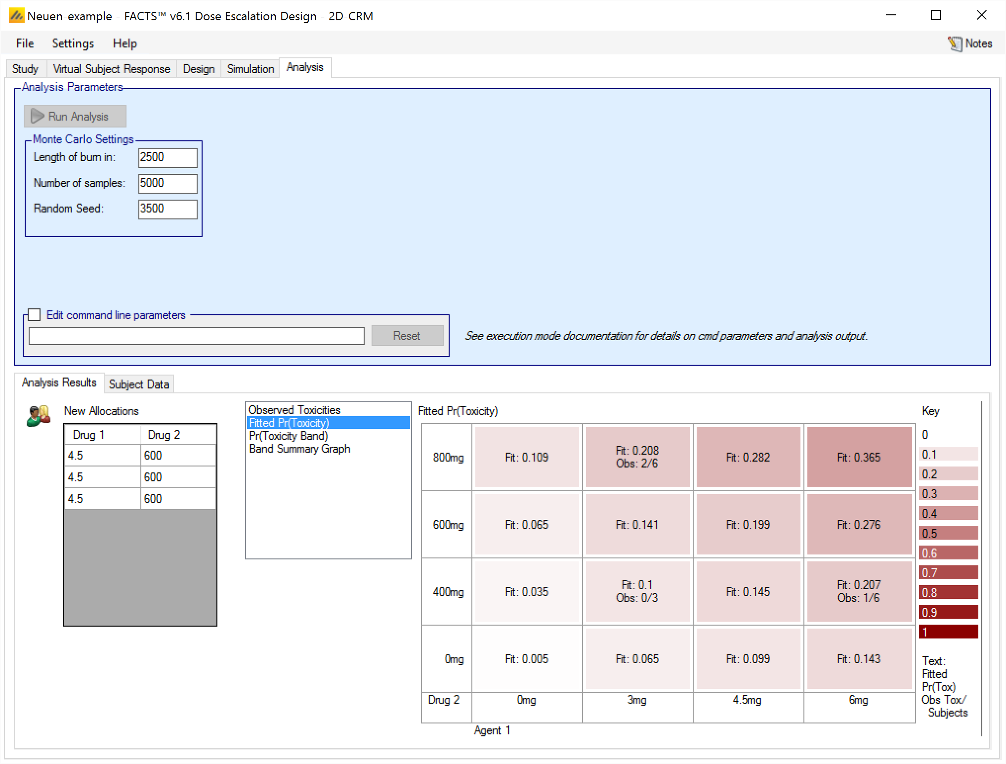
Fitted Pr(Toxicity)
This graph shows the mean fitted toxicity rate at each combination, colored with increasing intensity the higher the rate, and a summary of the observed data:
Pr(Toxicity Band)
This graph shows the posterior probability of being in a particular toxicity band at each combination, colored with increasing intensity the higher the probability, and a summary of the observed data:
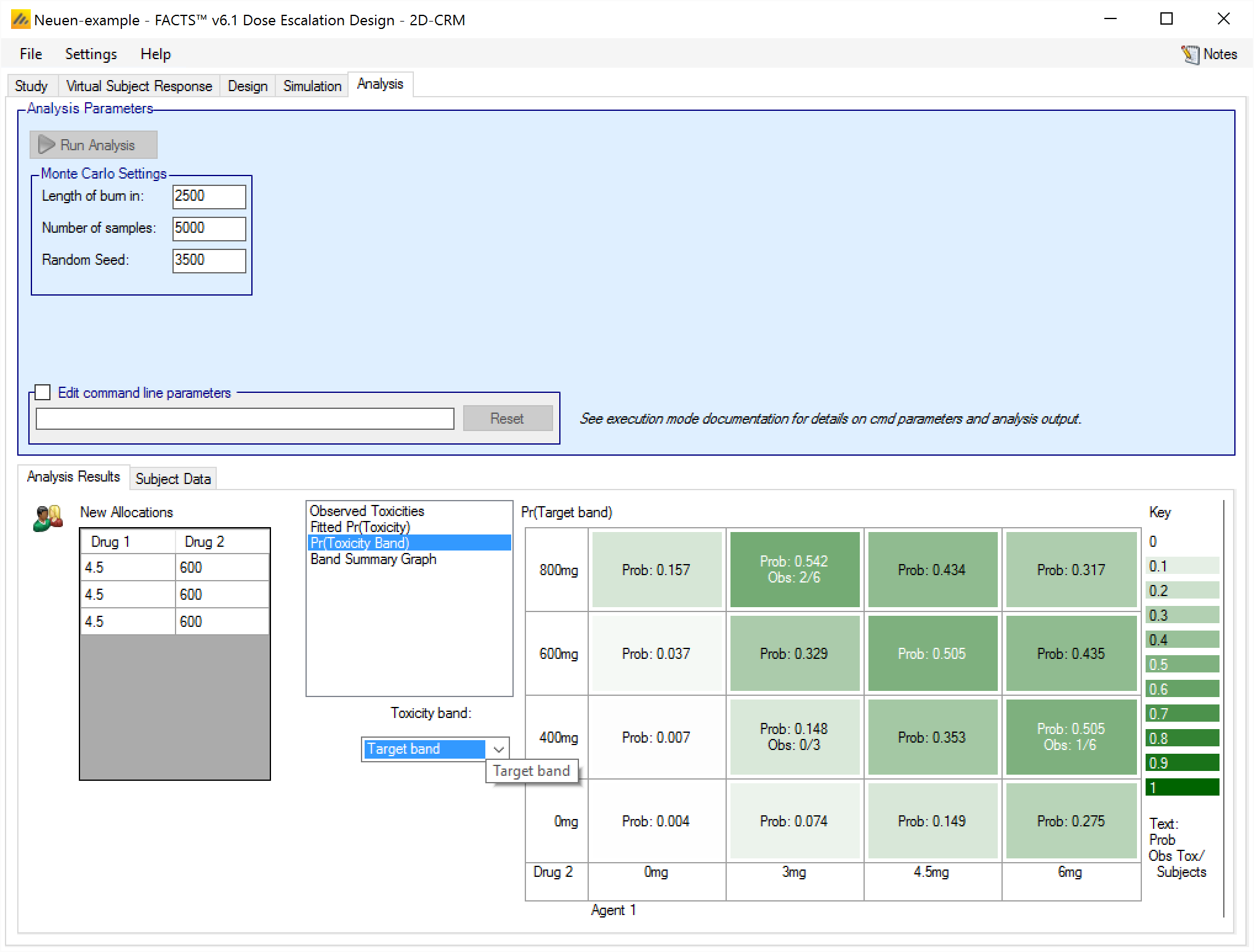
There is a control to select for which toxicity band the probabilities are shown.
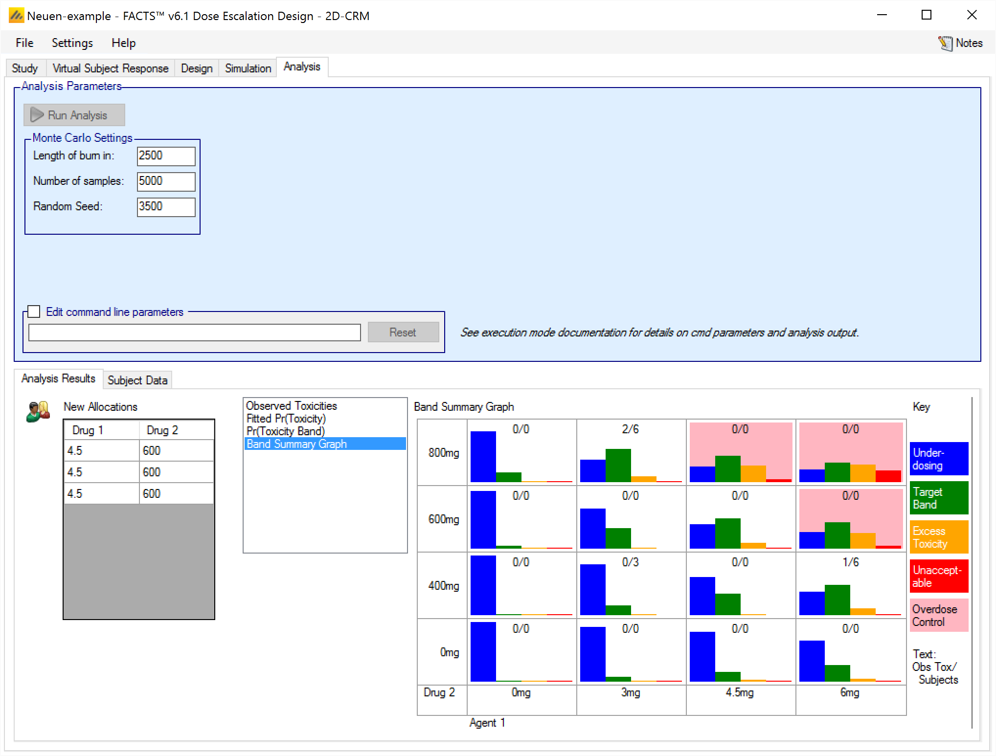
Band Summary Graph
This graph shows the posterior probability of being in each toxicity band at each combination as a simple histogram. Common y-axis range of 0-1 is used for all the histograms. The background of the histograms is white if the combination is within the overdose control rules and pink if the combination is excluded by the overdose control rules. At the top of each histogram is a summary of the observed data (toxicities / total observed):
The output files
For a description of the contents of the simulation results files, see the specification document [Spec]