Introduction

Purpose and Scope of this document

This document describes usage and how to utilize “R” to run FACTS. It is intended for anyone requiring posterior probabilities and decisions that FACTS does not include. It can be used to:

Simulate trials that require posterior quantities that FACTS does not include, e.g.:
1. The probability that a dose has a treatment effect in a certain range
Simulate trials that make decisions that FACTS does not include, e.g.:
1. Sample size re-assessment
2. Retain the dose meeting goal X and the next lowest dose

Warning: this process is not very forgiving of errors, nor very informative when they occur. It is recommended you start with the supplied example and then modify that in steps to the case you actually wish to analyze or simulate.

Calling FACTS from R

Software prerequisites

To call FACTS from R, you will need the following installed on your Windows machine on which you are using FACTS:

A reasonably recent version of R (v3.5.3+).
FACTS v6.4 or later, the command line executable versions of the FACTS simulation engines – these are currently available to Enterprise licensees.
The supplied R file: factR.R

factR.R

Provides an ‘R’ wrapper for accessing FACTS analysis models for:

Core and Enrichment Design, allowing you to use the following FACTS analysis features:
1. Dose Response models
2. Longitudinal models
3. Hierarchical Prior on Control (borrowing from historical data)
4. TTE predictor endpoint
5. BAC
Inputs
1. FACTS param file with trial info and model specifications
2. Data file
Output
1. MCMC file

Steps for calling FACTS from R

To call FACTS from R, you will need to do the following sequence of steps:

Create a (non-adaptive) FACTS project for your Engine type with the general study info: Number of Arms, number and timing of Visits (if using), Dose response (& longitudinal if using) model specification and MCMC setup.
Configure VSR and Execution profiles to allow a simple simulation run.
Run 1 simulation to produce:
1. A ‘param’ file which will be passed as an input to the R function.
2. A ‘patients’ file. This may be useful to illustrate data file format for the input data. See FACTS Execution Guides for details.
3. An ‘mcmc’ file. This will show you what to expect in the output MCMC file.
If using FACTS to analyze a data set, then
1. put the data set into the required format
2. write an R script to call FACTS with the data set
3. process the MCMC output
If using FACTS within a simulation framework, then:
1. Write an R script that generates the data you wish to simulate and pass to FACTS to analyze
2. Write a loop that
  - generates the data for a simulation
  - calls FACTS with generated data
  - process the MCMC output
  - accumulate the statistics for the overall operating characteristics to be computed
3. Output the resulting OCs

runFACTS() Usage Notes

Run FACTS MCMC Model from R

runFACTS(
 engine, 
 data.file = “patients.dat”, 
 param.file = “nuk1_e.param, 
 mcmc.file.num = 0, 
 rng.seed = 1, 
 exec.path = getwd()
)

Return Value: runFACTS returns a TRUE/FALSE to indicate a successful/failed execution. In case of errors, R error messages may be printed and in case of a FACTS execution error, a file called ‘error.txt’ will be output, containing the error description.

Arguments:

engine: Name of the FACTS engine to use. Can be one of the following:
1. For Core Engines: “contin”, “dichot”, “ME”, “TTE”
2. For Enrichment Design Engines: “ed_contin”, “ed_dichot”, “ed_tte”
data.file: Name of the input data file. Default is “patients.dat”. This file format should exactly match the file format of the ‘patients’ file corresponding to the ones produced by FACTS for the design you setup in FACTS to specify the analysis model. (See the FACTS Execution Guide under the FACTS Help menu for details.)
param.file: Name of the FACTS ‘.param’ file that specifies the model setup. Default is ‘nuk1_e.param’.
mcmc.file.num: The MCMC output is written to a file named ’mcmcNNNNN.csv. This argument set the NNNNN. Therefore, mcmc.file.num = 1 will create an MCMC output file called mcmc00001.csv. Default value is 0.
rng.seed: Integer-valued random number generator seed. Will use the value from the ‘.param’ file if unspecified.
exec.path The path to the directory where the FACTS executable program is available. Default is the current working directory.

Set Up Files and Folders

It is important to pass files and parameters correctly, as there is not much in the way of helpful error messaging. Setting up the required folder and files is not hard but should be done carefully. The following example shows how.

Example

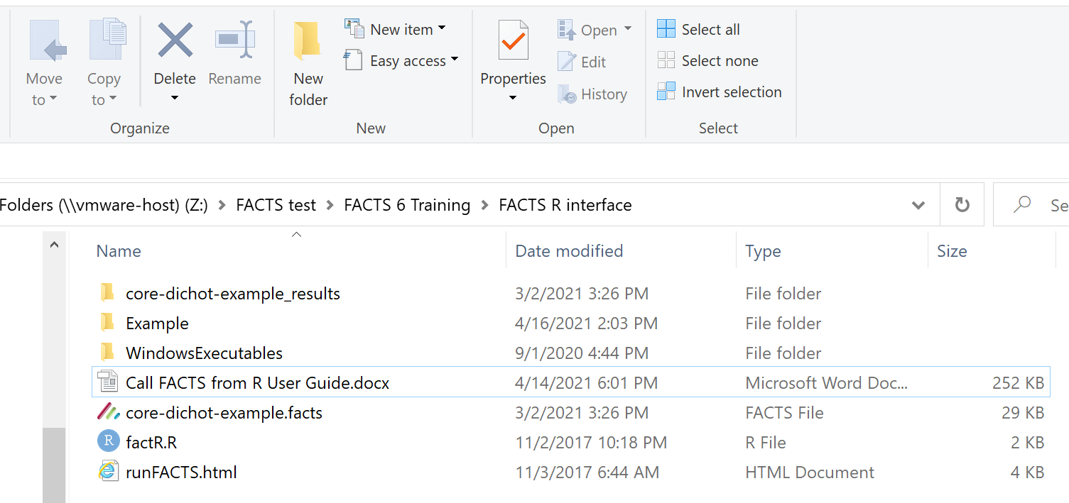
The paths and file names in the following examples are based on this example folder structure:

The top level folder containing

The folder “Example” where we will run FACTS.
The folder “WindowsExecutables” where the executable FACTS simulators are located.
The factR.R file.
The facts file “core-dichot-example.facts” use to generate the parameter file used in this example.
The folder “core-dichot-example_results” where we can find a parameter file once we have run a simulation.

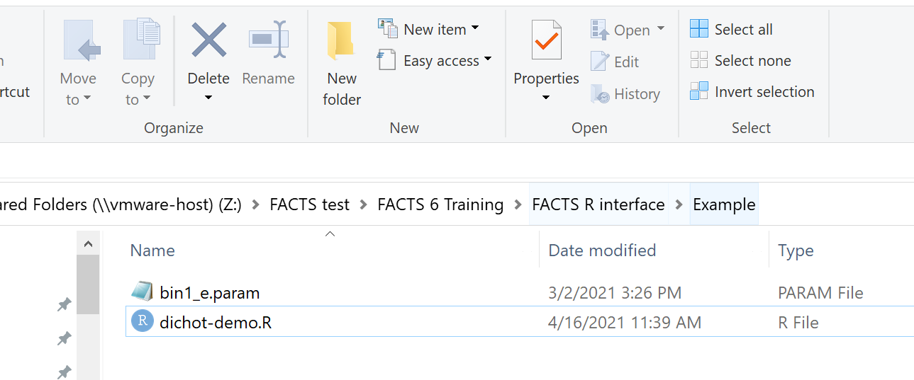
Within the Example folder there are just 2 files:

a copy of the facts parameter file from the example where we have defined the FACTS analysis to be performed,
the R file containing the code that will simulate our data, call FACTS and analyze the MCMC results.

“Example” is the folder where the parameter file and patient data must be located, and where the MCMC files are written. In our R session, we make it the working directory.

setwd(“z:/FACTS test/FACTS 6 Training/FACTS R interface/Example”)
The factR.R file is located in the parent folder:

FactR.src = “../factR.R”
The folder containing the FACTS executable files is in the parent folder:

Exec.dir = “../WindowsExecutables”

The “core.dichot.example.facts”

In this example we wish to use FACTS to fit a simple NDLM dose response model across 6 arms (control & 5 doses) with a dichotomous endpoint.

We have entered the following parameters:

Study:
- Study Info:
  - Non-adaptive
  - Recruit subjects continuously
  - Max subjects: 300
  - Response is a positive outcome
  - Time to final endpoint: 4 weeks
- Treatment Arms:
  - Control and 5 doses with strengths 1, 2, … 5
Virtual Subject Response
- Explicitly defined
  - Dose Response
    - responses: 0.1, 0.1, 0.125, 0.15, 0.2, 0.25
Execution
- Accrual
  - 1 region with mean accrual of 5 subjects per week
- Dropout
  - No dropouts
Quantities of Interest
- Posterior probability: Pr(P_d > P_Control)
- Probability of being target: Pr(Max)
- Decision Quantity: Pr(P_d > P_Contorl); d=Greatest Pr(Max)
Design
- Dose Response
  - Simple NDLM
    - Initial Dose ~N(0,2²)
    - Tau IG(1,1) “central value”, “weight”
- Requentist analysis: none
- Allocation: 1:1:1:1:1:1
- Success/Futility Criteria
  - Success: Pr(P_d > P_Control); d= Greatest Pr(Max) > 0.9

Not all these parameters will effect our analysis, but we have to enter sufficient parameters to be able to run a simulation and get a bin1_e.param file. This can be found in the scenario simulation results folder. We only need to run 1 simulation on order to have one written out. This file is copied to our “Example” directory. If we want to change something in the analysis – the model or the prior for example, we can modify this facts file, re-run one simulation, and copy the new bin1_e.param file.

dichot-demo.R

We start by setting the current working directory to the “Example” folder, and setting up some file locations and sourcing the factR.R file.

## Set up Folders and Paths

# This is the directory where the parameter file and patient data must be located
# It will be where the MCMCM files are written
setwd("Z:/FACTS test/FACTS 6 Training/FACTS R interface/Example")

# This must be the location of the factR.R file
FactR.src = "../factR.R"

# This must be the location of the executable files
Exec.dir = "../WindowsExecutables"

# Load runFACTS
source(FactR.src)

We can then copy an example patients file from the simulation results and check that we can run facts.

# Test to check its working
# Copy an example patients file from the simulations results to this folder before running.
system.time(
  runFACTS(
    engine='dichot', 
    data.file = 'patients00001.csv', 
    param.file = 'bin1_e.param', 
    mcmc.file.num = 1, 
    rng.seed = 1, 
    exec.path = Exec.dir
  )
)

genBinaryData()

We now define a simple function to generate the data for a single run of FACTS.

# generates a data frame that can be used to drive a FACTS analysis
# dichotomous endpoint
# no visits
# n.per.arm: int, the number of subjects to be simulated for each arm
# rates: int[], the response rate to be simulated for each arm
# the length if rates defines the number of arms
# returns a dataframe with n.per.arm * length(rates) simulated subjects

genBinaryData <- function(nPerArm, rates) {
  
  patientID <- 1:(nPerArm * length(rates)) # Generate a list of patients
  region <- rep(1, nPerArm * length(rates)) # all patients come from region 1
  date <- 1:(nPerArm * length(rates)) # Generate a list of enrolment dates - here simply one per day
  doseAlloc <- rep(1:length(rates), each = nPerArm) # Allocate patients equally to each dose
  lastVisit <- rep(1, nPerArm * length(rates)) # all patients have last visit data
  dropout <- rep(0, nPerArm * length(rates)) # no patients have dropped out
  baseline <- rep(-9999, nPerArm * length(rates)) # not simulating baseline
  visit1 <- rep(0, nPerArm * length(rates)) # create the outcome vector

  for (d in 1:length(rates)){ # get responses for each dose
  ix <- which(doseAlloc == d) # get indices of patients on dose d
  # assign them a final response based on the rate to simulate for dose d
  if (length(ix) > 0) {
  visit1[ix] <- 
    sample(
     c(0,1), 
     size = length(ix), 
      replace = TRUE, 
      prob = c(1-rates[d], rates[d])
    )
  }
  
}

dat <- data.frame(
  SubjectID = patientID, 
  Region = region, 
  Date = date, 
  Dose = doseAlloc, 
  LastVisit = lastVisit, 
  Dropout = dropout, 
  Baseline = baseline, 
  Visit1 = visit1, 
  row.names = NULL
)

return(dat)
}

runSims

########### Toy Example Trial Sim ##########
### Constants
DATAFILE = "patients.csv"
MCMCFILE = "mcmc00000.csv"
# function to simulate an example data set with dichotomous endpoint
# nSims - the number of sims to run
# nBurnin - the number of MCMC smaples to discard
# (the number of MCMC samples is specified in the parameter file)
# details - a boolean. If TRUE the function returns a data frame with
# the results of each individual simulation,
# otherwise just the win proportion and probabilities of being control

runSims <- function(
    nSims = 10, 
    nBurnin = 1000, 
    rates = c(0.1, 0.1, 0.125, 0.15, 0.2, 0.25),
    details = FALSE
) {

winPpn = 0
pr.gt.ctl.sum <- rep(0, length(rates) - 1)
if (details) {
perSim <- data.frame(Sim = 1)
}

for(sim in 1:nSims) {
dat = genBinaryData(nPerArm = 50, rates = rates)
write.csv(dat,DATAFILE, row.names = FALSE)
if (details) {
perSim[sim, "Sim"] <- sim
# record true rates and observed rates
for (d in 1:length(rates)) {
perSim[sim, paste("sim.rate.", d, sep="")] <- rates[d]
}

for (d in 1:length(rates)) {
perSim[sim, paste("obs.rate.", d, sep="")] <- mean(dat[dat[,"Dose"]==d, "Visit1"])
}
}

cat("run FACTS: ", sim, "\n")

ret <- 
  runFACTS(
    engine = 'dichot', 
    data.file = DATAFILE, 
    param.file = 'bin1_e.param', 
    mcmc.file.num = 0, 
    rng.seed = sim, 
    exec.path = Exec.dir
  )

dat = read.csv(MCMCFILE, skip = 1)

# discard burnin rows and just estimates of rate - the "Pi" columns
dat = dat[(nBurnin + 1):nrow(dat), grep("Pi", names(dat))]

if (details) {
# record est rate
for (d in 1:length(rates)) {
perSim[sim, paste("est.rate.", d, sep="")] <- mean(dat[,paste("Pi.", d, sep="")])
}
}

# success if the first dose is not in the top 2 .. i.e. the resposnse on any 2 doses is > control

success <- apply(dat, 1, FUN = function(x) {ifelse(length(x) - which(order(x)==1) >= 2, 1, 0)})

if (details) {
perSim[sim, "Pr.Success"] <- mean(success)
perSim[sim, "Success.flag"] <- ifelse(mean(success) > 0.9, 1,0)
}

winPpn = winPpn + ifelse(mean(success) > 0.9, 1,0)

# example: calc pr(theta_d > theta_ctl)
gt.ctl.flag <- apply(dat, 1, FUN = function(x){x[2:length(x)] > x[1]})
pr.gt.ctl <- apply(gt.ctl.flag,1,sum)
pr.gt.ctl <- pr.gt.ctl / length(gt.ctl.flag[1,])
pr.gt.ctl.sum <- pr.gt.ctl.sum + pr.gt.ctl

if (details) {
for (d in 1:length(pr.gt.ctl)) {
perSim[sim, paste("Pr.pi.", d+1, ">pi_ctl", sep="")] <- pr.gt.ctl[d]
    }
  }
}

cat("win proportion: ", winPpn/nSims, "\n")

if (details) {
return (list(winPpn/nSims, pr.gt.ctl.sum/nSims, perSim))
} else {
return (list(winPpn/nSims, pr.gt.ctl.sum/nSims))
}
}

Running the Example

Having sourced the above functions and variables holding paths and fllenames we can run the simulations with the default scenario:

runSims(details=FALSE)

> run FACTS: 1
> run FACTS: 2
> run FACTS: 3
> run FACTS: 4
> run FACTS: 5
> run FACTS: 6
> run FACTS: 7
> run FACTS: 8
> run FACTS: 9
> run FACTS: 10
> win proportion: 0.3

> [[1]]
> [1] 0.3

> [[2]]
> Pi.2 Pi.3 Pi.4 Pi.5 Pi.6
> 0.30572 0.45824 0.51936 0.77944 0.92916

If “details” is set to TRUE then the list of results has a dataframe at the end that contains a row per simulation and details of that simulations results.

Hopefully this is sufficient to get you started.