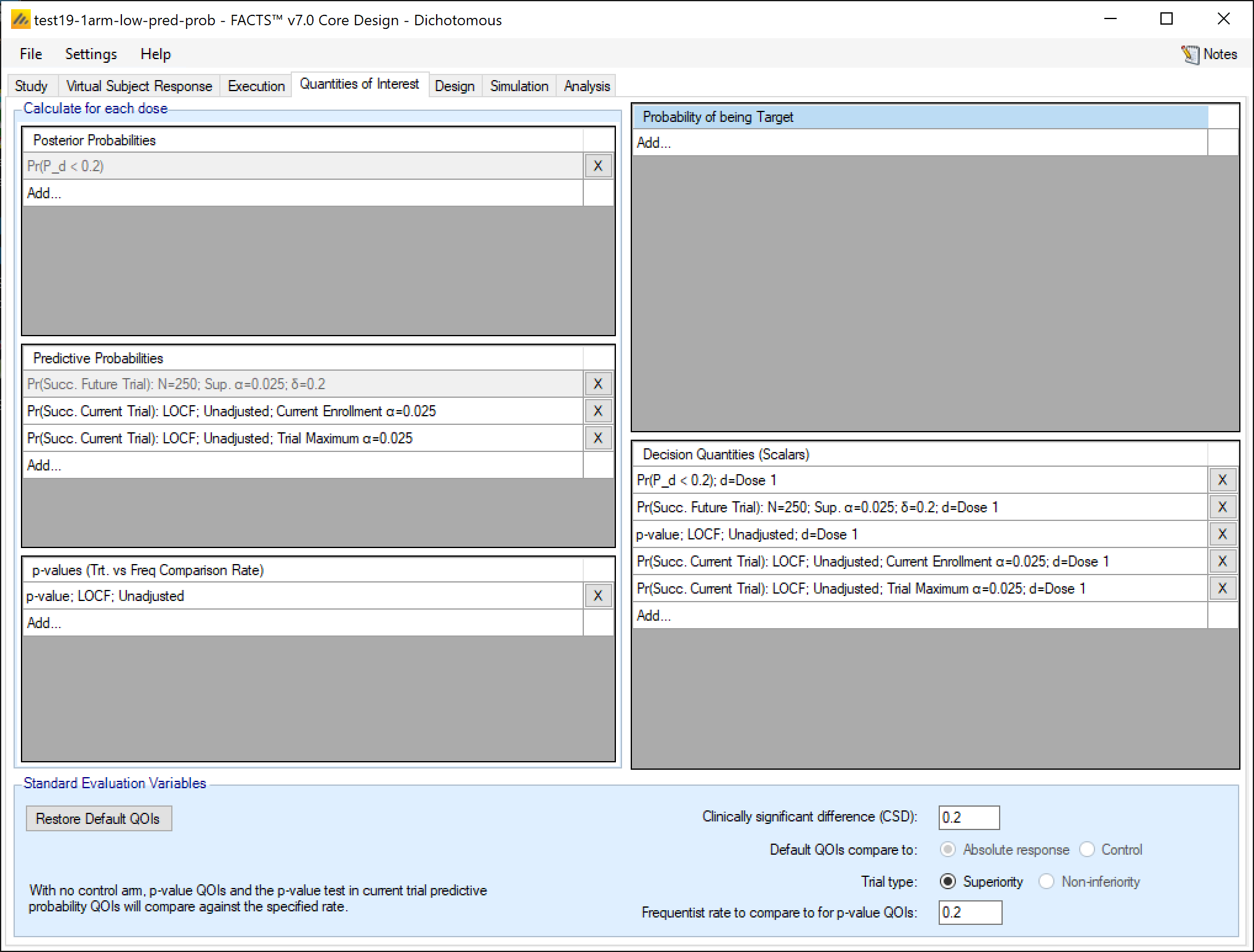
The QOI (Quantities Of Interest) tab allows the user to specify the Bayesian posterior quantities and frequentist p-values that are eligible to be used to make decisions in the trial as well as being output to the simulations results files.
There are 3 classes of QOI:
A probability calculated independently for each dose. There are 3 types of comparison:
The posterior probability that the estimate of the response of the subjects on that dose is better/worse than an absolute value or the estimate of response of the subjects on a reference dose, such as Control.
The predictive probability/conditional power of success (achieving frequentist statistical significance) in the current trial or a future trial comparing the estimate of response on the dose against that on the Control arm.
P-values for each dose comparing the estimate of response on that dose against that on the Control arm.
Probabilities calculated across the doses for which dose is most likely to satisfy a specified target dose criteria. The target dose criteria can be to determine the dose with the maximum effect (QOI is called Pr(Max)), the minimum dose that achieves some known minimum effect (called Pr(MED …)), or that it is the minimum dose that achieves some percentago of the effect estimated for the most effective dose (called Pr(EDq …) where \(q\) is the effect percentage).
A decision quantity – which is the value of either of the other types of QOIs at a specific dose level. The method of choosing the dose level that should be used for decision QOI is specified at the time of creating the decision QOI. As an example: a QOI may be created that calculates the Probability that each dose is superior to the control arm - Pr(PBO). Additionally, a target QOI can be created that calculates the probability that each dose is the ED90 - Pr(EDq relative to Control: Quantile=0.9). Then, a decision quantity could be created that is a scalar value representing the probability that the dose that is the most likely to be the ED90 is superior to control - Pr(\(\theta_d>\theta_{Control}\)); d=Greatest Pr(EDq relative to Control: Quantile=0.9). It is also easy to create a decision QOI that is simply the largest (or smallest) value of the dose specific QOI. An example of this would be the p-value of the dose with the smallest p-value.
Trial decisions at interim analyses or the final analysis are made based on decision quantities, but adaptations like adaptive allocation can be based on posterior probabilities, predictive probabilities, and target probabilities.
Note that to creating a QOI for early stopping or final evaluation decisions will involve using 2 or 3 QOIs:
The probability to be tested e.g. the probability of being better than the Control by a clinically significant difference.
The target dose criteria for selecting the dose that is to be used in the test – e.g. the ED90. This step is not always necessary.
The decision quantity that combines 1 & 2 – e.g. the probability that the ED90 is better than Control by a clinically significant difference.
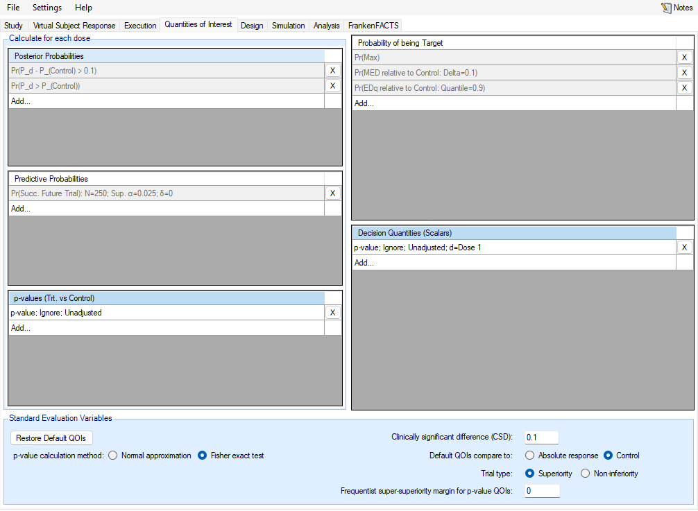
There are a number of pre-defined, default QOIs which simplifies the specification of the most commonly used decision quantities, and the importation of past FACTS designs. These are:
Default Posterior Probabilities
The probability of being better than the control arm: Pr(\(\theta_d > \theta_{Control}\)), previously referred to as Pr(\(\theta_d – \theta_0\)), Pr(Pbo) and Prob. Beats Ctrl in earlier versions of FACTS.
The probability of being better than the control arm by a clinically significant difference Pr(\(\theta_d - \theta_{Control} > \delta^*\))”, previously referred to as Pr(\(\theta_d – \theta_0 >\) CSD), Pr(CSD) and Prob. Beats CSD in earlier versions of FACTS. The value for the \(\delta^*\) is the CSD, which is set in the “Standard Evaluation Variables” panel at the bottom of the QOI tab.
Default Predictive Probabilities
- The probability of success in a future trial Pr(Succ. Future Trial): N=\(N_{Future}\), Sup/Noninf, \(\alpha=\alpha^*\); \(\delta=\delta^*\), previously referred to as Pr(S Phase III) and Prob. Stat Sig in earlier versions of FACTS. The parameters for the future trial can be modified from the default by clicking on the QOI’s row in the table.
Default Target Doses
The probability for each dose that it is the dose with the maximum response, Pr(Max), previously referred to as \(d_{max}\) and Ppn Max in earlier versions of FACTS. When used to select a dose in a decision quantity the label p… \(d\) = Greatest Pr(MAX) is used.
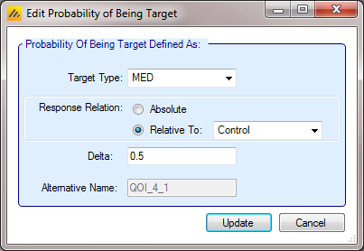
The probability for each dose that it is the minimum dose that is better than Control by the specified CSD, Pr(MED relative to Control: Delta = \(\delta^*\), previously referred to as Ppn (MED) in earlier versions of FACTS. The CSD used for comparison is specified in the Evaluation Variables panel at the bottom of the QOI tab. When used to select a dose in a decision quantity the label \(d\)= Greatest Pr(MED relative to Control/Active Comparator: Delta = \(\delta^*\)) is used.
The minimum dose that gives a certain proportion of the maximum estimated response Pr(EDq relative to Control: Quantile=\(Q\)), previously referred to as $d_{EDx} and Ppn(EDx) in earlier versions of FACTS. The Effective Dose quantile to use can be modified by the clicking on QOI’s row in the table. When used to select a dose in a decision quantity … \(d\)=Greatest Pr(EDq relative to Control: Quantile=\(Q\)) is used.
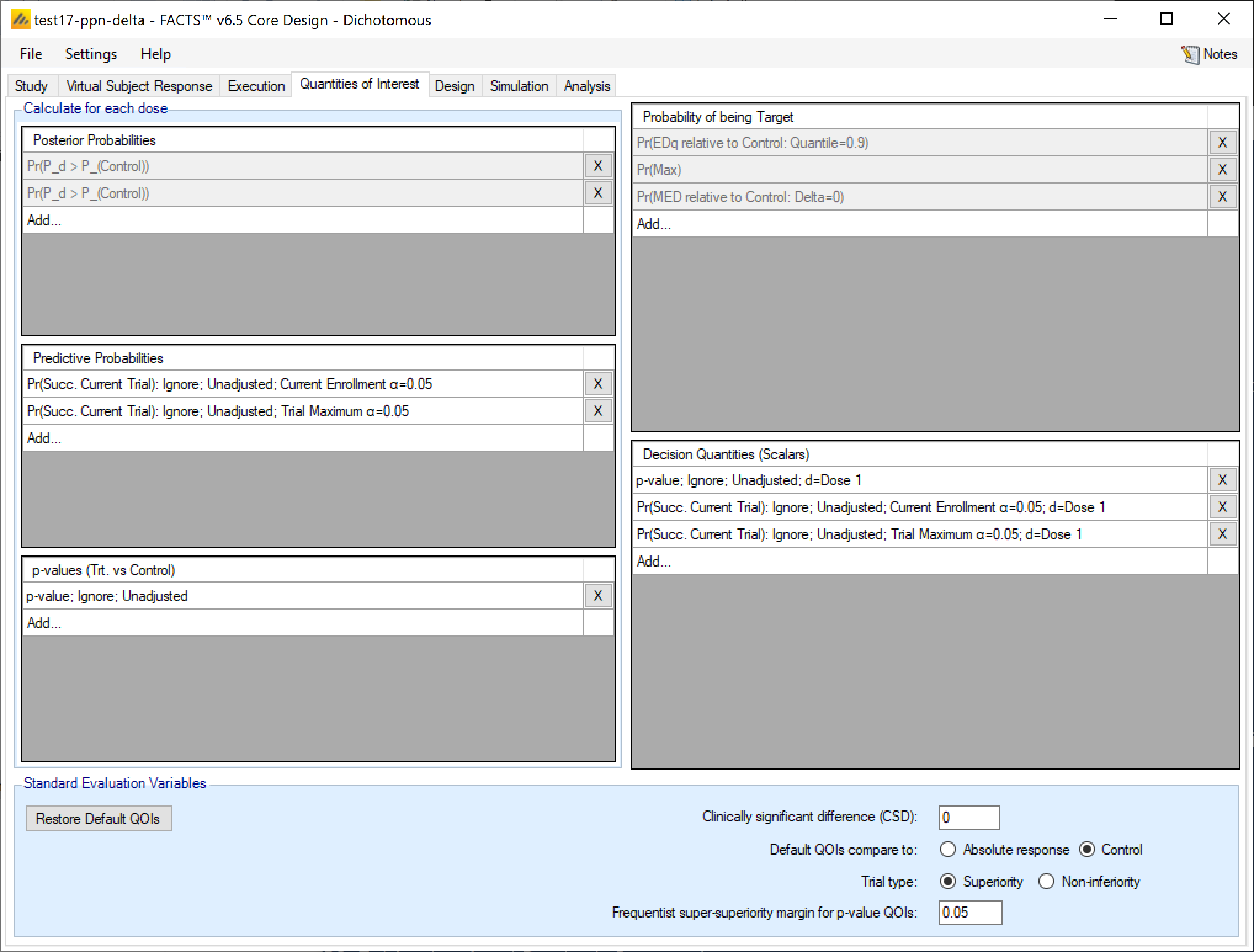
In each panel for each type of quantity, existing quantities can be deleted by clicking on the  at the end of the corresponding row. Each quantity’s definition can be displayed and edited (only edited for the default QOIs) by clicking on the row displaying the quantity’s definition. A new quantity can be defined by clicking on the bottom row of the corresponding panel labelled “Add…”.
Posterior Probabilities
These are Bayesian quantities to be calculated at each interim and at the final analysis.
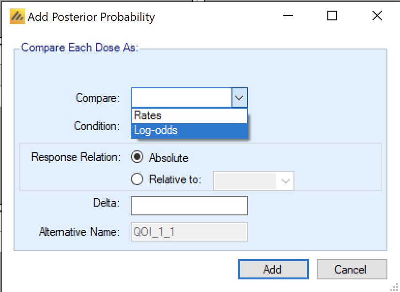
A Posterior Probability is specified by providing a value for each of the following:
Compare:
Continuous: Means
Dichotomous: Rates or Log-odds
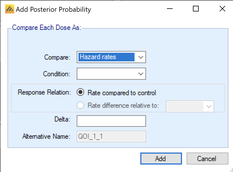
Time-to-Event: Hazard Ratio or Hazard Rates.
Condition: “>” or “<” a comparison value.
Relative to an absolute value or relative to the response on a specific dose.
The comparison can include a delta, which is the absolute value to be compared against if t the difference relative to the comparison arm is compared to. he comparison is absolute, or a value that
The QOI will be given a “name” derived from these details and a short or Alternative name that will be used in the output files to allow easier access from other software, e.g. from within R.
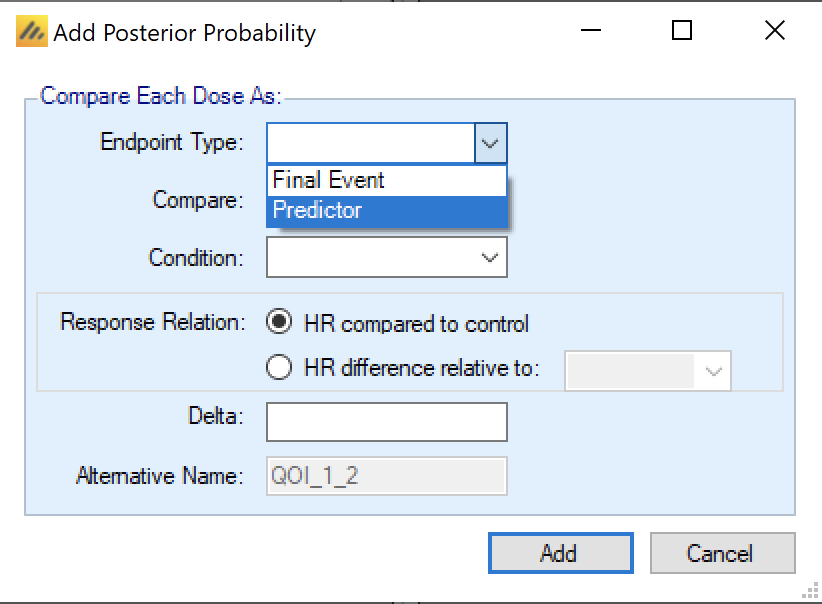
If the endpoint is TTE and the design includes a predictor endpoint, then the definition of the QOI includes the specification of which endpoint it applies to.
There are a couple of aspects of posterior probabilities that are slightly different for posterior probability QOIs.
First, in FACTS Core TTE a Posterior Probability QOI (a Bayesian comparison of estimates of response) can be used to compare Hazard Ratios or Hazard Rates. In their descriptions Hazard Ratio QOIs use “HR” (e.g. “HRd < 1”) and Hazard Rate QOIs use \(\lambda\) (e.g. “\(\lambda_d\) < \(\lambda_{control}\)”). If there are hazard rate QOIs defined, then FACTS restricts the hazard model (defined on the Design > Hazard Model tab) to use just a single segment (so that there is just one lambda to compare). This is set in the “Com are” box of the QOI definition window:
Additionally, in FACTS Core TTE when defining a Posterior Probability QOI (a Bayesian comparison of estimates of response) or a Target QOI (a Bayesian assessment of which treatment arm is most likely to fulfill a ‘target’ criteria) – the user can select whether the evaluation uses the Final Event endpoint, or the Predictor.
Notes on setting Deltas
For the three endpoint types, delta’s are defined as:
- Continuous
- A CSD (Clinically Significant Difference) in the estimates of the mean response.
- Dichotomous
- A CSD in the estimate of the response rates if Rates is selected in the QOI, and of log-odds of the response rate if Log-odds is selected in the QOI.
- Time-to-Event
- A CSHRD (Clinically Significant Hazard Ratio Difference) in the estimate of the Hazard Ratio
A standard hypothesis test for demonstrating superiority to control uses a delta of 0. Testing for superiority with a non-zero delta is different, and the implications need to be carefully understood Simulating its use in FACTS is a good way to achieve that understanding! . Where the term CSD is used in this document, it should be taken to refer to CSHRD as well unless it is specifically stated otherwise.
When setting a target treatment difference from control for the study to beat, it is also common to require a degree of confidence that the target has been beaten. To achieve posterior probabilities of >50% that the target has been beaten, the estimated mean difference will have to be greater than the target difference.
Thus, when setting a delta, we are setting up two hurdles the study drug must beat, first the delta and then on top of that an additional margin to give a >50% confidence that the margin has been beaten. Thus, it is necessary to avoid setting the target delta too large. A common mistake is to set the delta to the ‘expected difference’ (the value that might have been used in a conventional sample size calculation). In scenarios where the simulated response is equal to the ‘expected difference’ and hence the CSD this will give probabilities of being better than control by the delta of 50% on average, regardless of the sample size.
It is inadvisable to require a posterior probability of 50% that the response is better than the Control by the delta margin as this turns the test into one that simply depends on whether the point estimate of the response is better.
It is inadvisable to require posterior probability of less than 50% for success, as such criteria have the undesirable characteristic that they can be met in circumstances where it can be seen that if further data was gathered consistent with what has already been seen, it would lead the threshold no longer being met! The posterior distribution would shrink so that there was no longer sufficient of the tail above the CSD.
It is better therefore to use a delta that is less than the expected difference that it is hoped to achieve, somewhat like having a non-inferiority margin around the target. So, when the design is simulated with a response at the expected difference the target will be clearly exceeded. A useful default value to use for a delta is half the ‘expected difference’. This usually yields “comprehensible” probability thresholds for both success and futility.
Using a delta has benefits however – simply being better than control but for very small difference can be established simply by having large sample sizes. Being better than control by a delta establishes some confidence that there is some patient benefit. Use of a delta is also useful if otherwise success thresholds “well out in the tail” (e.g. > 0.99) are required such as the equivalent of an early look in a conservative Group Sequential design. Though the use of a delta does mean that there is a less direct equivalence to a p-value.
P-value Delta’s
Separately from the CSD/CSHRD delta, with a continuous or dichotomous endpoint (but not time-to-event), a frequentist super-superiority/non-inferiority delta can be specified.
These use the same selection of super-superiority/non-inferiority as the CSD
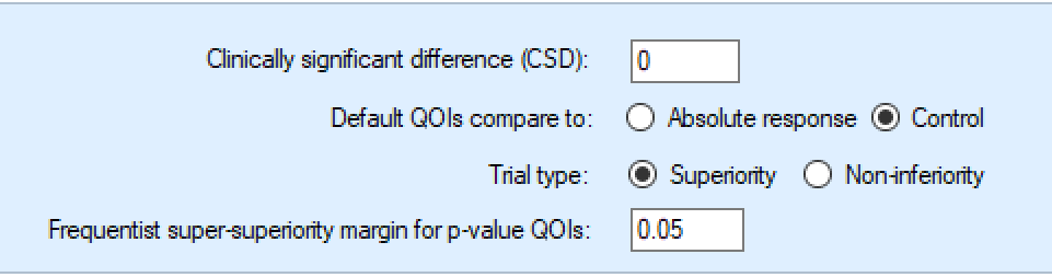
Currently, unlike the CSD delta that is only applied to the default posterior probability QOI and MED target QOI, the p-value delta is applied to all the p-value QOIs and it cannot be overridden.
The value of the p-value delta is constrained to be 0 or positive. The ‘direction’ of the delta depends then on the direction of the endpoint (whether “higher/lower is better” or “a response is a positive/negative outcome”).
| Higher is better / Response is positive | Lower is better / Response is negative | |
|---|---|---|
| Super-Superiority | Trt – Control > delta | Trt – Control < -delta |
| Non-inferiority | Trt – Control > -delta | Trt – Control < delta |
P-value Comparisons with No Control Arm
If no control arm is included p-values, with a continuous or dichotomous endpoint, the treatment response is compared to a fixed value. The fixed value is specified as “Frequentist response/rate to compare to for p-value QOIs:” in the Standard Evaluation Variables section at the bottom of the QOIs tab. It is not currently possible to compare different p-value QOIs to different fixed responses or rates.
Predictive Probabilities
There are two types of predictive probabilities –
Bayesian predictive probabilities, which are Bayesian predictions of frequentist outcomes and take into account the uncertainty around a set of parameters, and
Conditional Power, which aims to calculate the frequentist probability of success assuming a set of parameters to be true.
The primary difference between the Bayesian predictive probabilities and the conditional power calculations is that the Bayesian predictive probabilities are calculated taking the variability around the estimated treatment effect into account, while the conditional power calculations assume that the observed test statistic of past data is the exact effect that future data will be generated from.
For both Bayesian predictive probabilities and conditional power, we differentiate two types, predicting the outcome in the current trial and predicting the outcome in a future trial.
Bayesian predictive probabilities
Current Trial Bayesian Predictive Probabilities
In the current trial, the outcome can be predicted under one of two assumptions:
That no new subjects are recruited, but all those who have been recruited are followed up until they are complete.
That the trial continues recruiting using the current allocation ratios until the trial maximum sample size is reached, and all subjects recruited are followed up until complete.
Predictive probabilities currently can only predict outcomes based on p-values. Note that since p-values are only calculated as comparisons against a control arm, predictive probabilities of success in the current trial are only available if the current trial includes a control arm.
The user specifies how missingness is handled in the final analysis, the p-value test type – unadjusted, Bonferroni or Dunnett’s (Dunnett 1955) and the (one sided) alpha level for the significance test. The QOI assumes that the specified default p-value delta is used in the final test.
The predictive probability of the current trial at the maximum sample size is only available:
- If the allocation is either fixed, or fixed with arm dropping, but not adaptive allocation.
The predictive probability is calculated by simulating the remaining subjects, assuming their allocated at the current probabilities of allocation and simulating their final response based on the rate of response or (Normal) distribution of responses observed so far for each arm.
Ignoring the possibility of the trial stopping or dropping an arm at a future interim
Ignoring the possibility of future subject drop-outs.
There is one simulation of the remaining data per MCMC loop, potentially significantly increasing the time to perform the overall simulation of the trial.
If there is no data available on the arms involved in the Bayesian predictive probability calculation, FACTS will still perform the simulation of future subject outcomes based on posterior distribution. The posterior distribution for the arms with no available data will be the same as the user specified prior distribution.
Current Trial Bayesian Predictive Probabilities – Time-to-Event
Unlike the Continuous and Dichotomous endpoints, to predict the probability of success at full enrollment with a Time-to-Event endpoint, it is also necessary to simulate the accrual rate (and hence how many events might be observed).
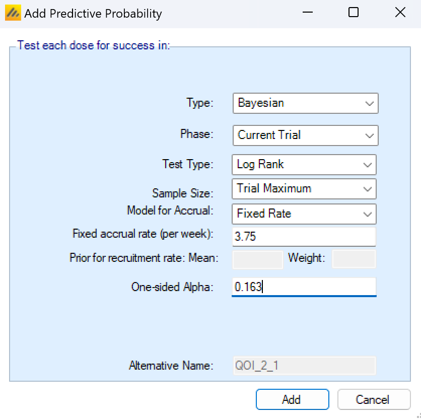
For TTE, for a Predictive Probability of Success at Full Enrollment, there are new parameters to determine how accrual is modeled. There are 3 models for accrual
Fixed Rate, the parameters for this are:
- The fixed (mean) accrual rate per week to simulate.
Estimated from the Last ‘W’ Weeks accrual data, using a Poisson distribution, with a Gamma prior. The parameters for this are
The number of past weeks W to use the accrual data from.
The prior mean for the model of the accrual rate
The weight of the prior
Estimated from all the accrual data from the start of the trial, using a Poisson distribution, with a Gamma prior, the parameters for this are:
The prior mean for the model of the accrual rate
The weight of the prior
Future Trial Bayesian Predictive Probabilities
For predictive probabilities for a future trial, a predictive probability of success in a subsequent phase 3 trial is estimated during the current trial. The probability of success in phase 3 is calculated for each study arm, based on the specification of the phase 3 trial given here of:
whether the aim is to show superiority or non-inferiority,
the sample size per arm,
the required one-sided alpha,
and the super-superiority margin or non-inferiority margin (if any).
Given these criteria, FACTS calculates the predicted probability of success of the subsequent trial for that endpoint assuming the estimate of the response on that endpoint, integrated over the uncertainty in those estimates. The conventional expected power of the specified future trial is calculated for the treatment effect in each MCMC sample and then averaged. This predicted probability of success can then be used in the stopping criteria and final evaluation criteria for the current trial.
This QOI is an extension of the “probability of success in phase 3” in earlier versions of FACTS – the difference now is that multiple different possible future trials can be specified in different QOIs and used for different decisions.
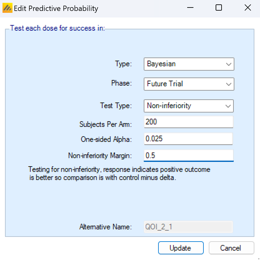
This predictive probability has the following parameters that must be specified:
Whether the future trial will be for Superiority or Non-inferiority.
The size of the future trial in terms of the number of subjects on each arm.
The (one sided) alpha level that will be used to determine the significance of the trial.
The Super-superiority margin (if any) or the non-inferiority margin. The default p-value delta is not used for this QOI it is specified as part of the QOI and can be different from the default.
As with all QOIs, the future trial predictive probability QOI will be given an alternative shorter name that can be used when accessing the output files from other software such as R.
If there is no data available on the arms involved in the Bayesian predictive probability calculation, FACTS will still calculate the predictive probability of the future trial being a success based on the estimated posterior distribution. The posterior distribution for the arms with no available data will be the same as the user specified prior distribution.
Conditional Power
Conditional power is currently available for Continuous and Dichotomous endpoints in Core and Staged Designs.
When creating a Conditional Power QOI, the first specification that must be made is whether the conditional power should be calculated for the current trial or for a hypothetical future trial. The two selections are fundamentally different.
The Current Trial conditional power takes the information collected in the trial so far, and assumes that for the remainder of the current trial the data collected has an effect equal to the point estimate of the already collected data. The previously collected trial data is then combined with hypothetical future data and weighted based on the amount of information that has been and will be observed by the end of the trial. The result is the probability that the current trial will reject the null hypothesis at a provided alpha level under the assumption that the future patients are generated from a population having a treatment effect exactly equal to the past data’s test statistic.
The Future Trial conditional power also uses the information accrued in the trial so far to calculate the assumed treatment effect moving forward, but assumes that a new study would be started that does not use the data from the current trial in its analysis. The new study is assumed to be a 1:1 randomized study if there is a control arm, and a single arm study if no control, with a sample size per arm, objective, and alpha level specified at the time of QOI creation.
If a conditional power is ever calculated for an arm with no final response data or against a control arm with no final response data, the conditional power will be called missing (-9999 in FACTS).
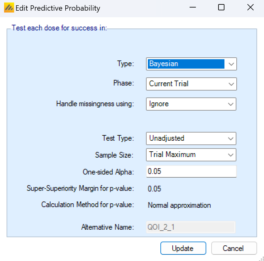
Current Trial Conditional Power
When creating a current trial conditional power, the missingness strategy, multiplicity adjustment, final sample size, and alpha level for the significance test must be specified.
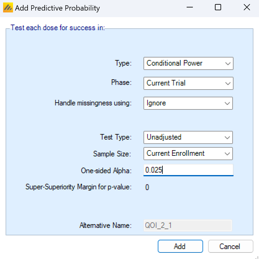
Handle missingness using:
Missingness handling for a continuous endpoint can be specified as:
Ignore: subjects that are known dropouts are not included in the current or final sample size, and are not used to estimate the treatment effect.
Last Observation Carried Forward (LOCF): subjects that are known dropouts have their last observed endpoint value assumed to be their final endpoint. Subjects with no early observed data are ignored. Subjects that have data to carry forward are considered complete, and are used to estimate the current treatment effect.
Baseline Observation Carried Forward (BOCF): subjects that are known dropouts have their baseline value assumed to be their final endpoint. They are included in the current information as complete subjects and are used to estimate the current treatment effect. BOCF is only available for the continuous endpoint and when simulating baseline for subjects.
Failure: subjects that are known dropouts are assumed to have a negative outcome at their final visit. If responses are good, the subject is a non-response, and if responses are bad, the subject is a responder. Failure is only available for dichotomous endpoints.
Test Type
The test type can either be Unadjusted or Bonferroni. An unadjusted test will always use the specified alpha level in the significance test. The Bonferroni adjustment will divide the specified alpha value by the number of non-control arms enrolling in the study in the enrolment period leading up to the current analysis time.
Sample Size:
The current trial conditional power can be calculated at two different future time points.
Current Enrollment: That no new subjects are recruited, but all those who have been recruited are followed up until they are complete.
Trial Maximum: That the trial would continue recruiting subjects using the current allocation ratios until the trial maximum sample size is reached, and all subjects recruited are followed up until they have the opportunity to complete.
One-sided Alpha
The threshold that the current trial would have to be less than in order to be considered a success. The success/futility values specified in the design tab are not used in the conditional power calculation. This value may be adjusted by the “Test type:” input.
Super-Superiority (Non-inferiority) margin for p-value:
This value cannot be changed on the QOI pop-up. It’s instead modified at the bottom of the QOI page. The objective of the current trial cannot be different for each individual current trial conditional power QOIs.
Additional Notes
Currently, conditional power will always assume that there is no correction applied to combine the different p-values from the analysis timepoints, i.e. no combination test is used.
The conditional power of the current trial at the maximum sample size is only available if the allocation is either fixed, or fixed with arm dropping, but not adaptive allocation or deterministic allocation.
Conditional power for the current trial is calculated
Ignoring the possibility of the trial stopping or dropping an arm at a future interim
Ignoring the possibility of future subject drop-outs.
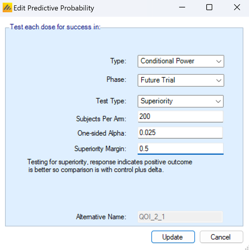
Future Trial Conditional Power
Conditional power of a future trial is reduced to a power calculation for a future trial, given the current frequentist estimates of treatment effect and standard deviation and a set of assumptions for the future trial, such as sample sizes, hypothesis to be tested, and significance levels to be used.
The test type of the future trial can be set to Superiority or Non-inferiority. If the superiority or non-inferiority margin is set to 0, then both types of tests simplify to traditional tests of superiority with no margin. If a non-zero margin is set, then the future trial must meet the success criteria indicated by the test type and the margin. The margin cannot be negative, but a super superiority test with a margin of -0.5 is equivalent to a non-inferiority test with a margin of 0.5.
The subjects per arm dictates how many subjects would be enrolled on each arm in the future study. If there is a control arm in the current trial, then the future trial is assumed to be randomized 1:1 between the active arm and the control. If there is no control arm in the current study, then the future trial is a single arm trial testing against the performance goal specified in the Freq. Comparison Response box in the QOI creation pop-up.
The One-sided Alpha is the significance level of the final analysis test of the future trial. The future trial is assumed to have 1 active arm, so there are no adjustments to the alpha level available.
The superiority margin or non-inferiority margin indicate the amount that the active arm must be better/not worse than the control arm by. If there is no control arm then this is the Freq Comparison response, which is the value that the active arms must be significantly better than in order to be declared a success. The frequentist margin for p-value QOIs on the QOI tab is not used for Future conditional power calculations – the future trial can have a different objective than the current trial.
Technical Aspects of Conditional Power Calculations
The conditional power calculations in FACTS are all calculated similarly to Jennison and Turnbull (2000).
For continuous endpoint conditional power calculations, the conditional power of the future trial is calculated using a pooled standard deviation from all arms. For dichotomous conditional power calculations, each arm has its own standard deviation based on the MLE estimate of its proportion. These decision result in the conditional power tests matching how standard p-value QOIs are calculated for continuous and dichotomous endpoints.
The following sections will provide formulae to calculate the conditional power in the case where there is a control arm. Simplifications for when the arm is being compared to a fixed value rather than a control arm are trivial: information fractions are only a function of the active arm standard deviation and the test statistic does not have a second sample mean subtracted from the active arm.
The value of \(\delta\), which can be a non-inferiority margin or a super superiority margin, is always positive coming out of FACTS. To make the math more concise we can define a couple of coefficients for the \(\delta\) term that allow it to be used without re-writing formulas for different hypothesis test setups. If high values of the endpoint are good, then \(s_1 = 1\), and if low values of the endpoint are good, then \(s_1=−1\). If the specified \(\delta\) is a non-inferiority margin, then \(s_2 = 1\), and if it’s a super superiority margin then \(s_2=-1\).
Continuous Conditional Power for the Current Trial
Let t be the interim index that the conditional power is being computed at, and T be the time of the analysis that the conditional power is being computed for. Then \(Z_k\) is the test statistic of the data collected up to the current interim analysis in the study, \(I_k\) is the information level at the time of the interim analysis, and \(I_K\) is the information level at the end of the study that the conditional power is being calculated for.
Let arm 1 be the control and arm 2 be the active arm, \(\bar{x_{it}}\) be the sample mean of arm \(i\) at time \(t\), \(\widehat{\sigma_{i}^{2}}\) be the sample variance of arm \(i\) at time \(t\), \(n_{it}\) be the number of subjects with complete known final data on arm \(i\) at interim analysis \(t\), and \(n_{iT}\) be the number of subjects with complete known final data on arm \(i\) at the time that conditional power is being calculated for. The pooled variance estimate is \(\widehat{\sigma^{2}} = \sum_{d = 1}^{D}\widehat{\frac{\sigma_{d}^{2}}{n_{dt}}}\) where D is the total number of arms in the study.
Then,
\[I_{t} = \left( \frac{\widehat{\sigma^{2}}}{n_{1t}} + \widehat{\frac{\sigma^{2}}{n_{2t}}} \right)^{-1}\]
\[I_{T} = \left( \frac{\widehat{\sigma^{2}}}{n_{1T}} + \widehat{\frac{\sigma^{2}}{n_{2T}}} \right)^{-1}\]
\[Z_{t} = \left( {\overline{x}}_{2t} - {\overline{x}}_{1t} + s_{1}s_{2}\delta \right)\sqrt{I_{t}}\]
where \(\delta\) is the non-inferiority or super superiority margin.
Then for a one-sided alpha level of \(\alpha\), let \(Z_{1-\alpha}\) be the critical value corresponding to \(\alpha\).
If high values of the endpoint are good, the conditional power of the current trial is:
\[CP_{T} = \Phi\left( \frac{Z_{t}\sqrt{I_{t}} - z_{1 - \alpha}\sqrt{I_{T}} + ({\overline{x}}_{2t} - {\overline{x}}_{1t} + s_{2}\delta)\left( I_{T} - I_{t} \right)}{\sqrt{I_{T} - I_{t}}} \right)\]
If low values of the endpoint are good, the conditional power of the current trial is:
\[CP_{T} = \Phi\left( \frac{{- Z}_{t}\sqrt{I_{t}} - z_{1 - \alpha}\sqrt{I_{T}} - ({\overline{x}}_{2t} - {\overline{x}}_{1t} - s_{2}\delta)\left( I_{T} - I_{t} \right)}{\sqrt{I_{T} - I_{t}}} \right)\]
Calculation of Continuous Conditional Power for a Future Trial
Most of the future trial conditional power calculation is the same as the above current trial conditional power. There are some simplifications.
\({\overline{x}}_{it}\) and \(\widehat{\sigma_{i}^{2}}\) are the same as in the current conditional power calculation. \(I_t\), the weight of the current trial Z-score, is set to 0. \(I_T\) is now the information at the end of the future trial, and is calculated as:
\[I_{T} = \left( \frac{\widehat{\sigma^{2}}}{n_{T}} + \widehat{\frac{\sigma^{2}}{n_{T}}} \right)^{- 1}\]
where \(n_T\) is the sample size per arm in the future trial and again \(\widehat{\sigma^{2}}\) is the pooled variance.
If high values of the endpoint are good, the conditional power of a future trial is:
\[CP_{T} = \Phi\left( \frac{- z_{1 - \alpha}\sqrt{I_{T}} + ({\overline{x}}_{2t} - {\overline{x}}_{1t} + s_{2}\delta)\left( I_{T} \right)}{\sqrt{I_{T}}} \right)\]
If low values of the endpoint are good, the conditional power of a future trial is:
\[CP_{T} = \Phi\left( \frac{- z_{1 - \alpha}\sqrt{I_{T}} - ({\overline{x}}_{2t} - {\overline{x}}_{1t} - s_{2}\delta)\left( I_{T} \right)}{\sqrt{I_{T}}} \right)\]
Calculation of Dichotomous Conditional Power for the Current Trial
The dichotomous conditional power calculations are similar in spirit to the continuous conditional power calculations. One substantial difference is in how the dichotomous conditional power tests handle a non-inferiority or super superiority margin, \(\delta\). The method of calculating an appropriate test statistic for a frequentist hypothesis test is not obvious when the null scenario has a non-zero \(\delta\).
When there is no margin, the estimate for each treatment is simply based on the observed response proportion \(\widehat{p_{i}}\) for arm \(i\), and the test statistic for a comparison of the control arm, \(c\), with dose \(d\) is the usual Wald test
\[Z_{d} = \frac{\widehat{p_{d}} - \widehat{p_{c}}}{\sqrt{\frac{\widehat{p_{d}}(1 - \widehat{p_{d}})}{n_{d}} + \frac{\widehat{p_{c}}(1 - \widehat{p_{c}})}{n_{c}}}}\]
When there is a margin, FACTS uses the Farrington-Manning Likelihood Score test statistic to estimate quantities \(\widetilde{p_{d}}\) and \(\widetilde{p_{c}}\) based on the MLEs of the arm proportions governed by the constraint that \(\widetilde{p_{d}} - \widetilde{p_{c}} = - s_{1}s_{2}\delta\). These constrained MLE estimates are used in the standard error of the test statistic. The FM test statistic is then,
\[Z_{FM,d} = \frac{\widehat{p_{d}} - \widehat{p_{c}} + s_{1}s_{2}\delta}{\sqrt{\frac{\widetilde{p_{d}}(1 - \widetilde{p_{d}})}{n_{d}} + \frac{\widetilde{p_{c}}(1 - \widetilde{p_{c}})}{n_{c}}}}\]
See the PASS documentation (NCSS 2025) or the SAS documentation (SAS Institute 2016) for a complete description of the calculations that go into the FM test. In the SAS documentation, note that the FM test is the same as the Miettinen-Nurminen test without including the \(\frac{n}{n - 1}\) variance correction. The FM test was used rather than the MN test because as \(\delta \rightarrow 0\), the FM test converges to the simple Wald test.
Once the test statistic has been resolved, the dichotomous conditional power for the current trial is calculated as follows. For calculating the conditional power for arm 2 compared to the control arm, called arm 1 without loss of generality, let \(I_t\) be the current information amount and \(I_T\) be the amount of information that the conditional power is being calculated for. Then,
\[I_{t} = \left( \frac{\widetilde{p_{1}}\left( 1 - \widetilde{p_{1}} \right)}{n_{1t}} + \frac{\widetilde{p_{2}}\left( 1 - \widetilde{p_{2}} \right)}{n_{2t}} \right)^{- 1}\]
\[I_{T} = \left( \frac{\widetilde{p_{1}}\left( 1 - \widetilde{p_{1}} \right)}{n_{1T}} + \frac{\widetilde{p_{2}}\left( 1 - \widetilde{p_{2}} \right)}{n_{2T}} \right)^{- 1}\]
\[Z_{t} = \left( \widehat{p_{2}} - \widehat{p_{1}} + s_{1}s_{2}\delta \right)*\sqrt{I_{t}}\]
where \(\delta\) is the super superiority or non-inferiority margin, and \(n_{1t}\) and \(n_{2t}\) are current number of completers on the control and active arm, and \(n_{1T}\) and \(n_{2T}\) are the number of completers that will be on the control and active arm at time that the conditional power is being calculated for. Additionally, if there is no non-inferiority or super superiority margin \(\delta\), then all \(\widetilde{p_{*}}\) values are equal to their corresponding \(\widehat{p_{*}}\) values.
For a one-sided alpha level of \(\alpha\), let \(z_{1-\alpha}\) be the critical value corresponding to \(\alpha\).
If high values of the endpoint are good, the conditional power of the current trial is:
\[CP_{T} = \Phi\left( \frac{Z_{t}\sqrt{I_{t}} - z_{1 - \alpha}\sqrt{I_{T}} + (\widehat{p_{2}} - \widehat{p_{1}} + s_{2}\delta)\left( I_{T} - I_{t} \right)}{\sqrt{I_{T} - I_{t}}} \right)\]
If low values of the endpoint are good, the conditional power of the current trial is:
\[CP_{T} = \Phi\left( \frac{{- Z}_{t}\sqrt{I_{t}} - z_{1 - \alpha}\sqrt{I_{T}} - (\widehat{p_{2}} - \widehat{p_{1}} - s_{2}\delta)\left( I_{T} - I_{t} \right)}{\sqrt{I_{T} - I_{t}}} \right)\]
Calculation of Dichotomous Conditional Power for a Future Trial
Most of the calculation quantities for the future trial conditional power are the same as the current trial conditional power. The only difference is that for the future trial conditional power we discard the influence of the current trial test statistic on the final analysis, so \(I_t=0\). Then the conditional power calculations become:
If high values of the endpoint are good, the conditional power of a future trial is:
\[CP_{T} = \Phi\left( \frac{- z_{1 - \alpha}\sqrt{I_{T}} + (\widehat{p_{2}} - \widehat{p_{1}} + s_{2}\delta)\left( I_{T} \right)}{\sqrt{I_{T}}} \right)\]
If low values of the endpoint are good, the conditional power of a future trial is:
\[CP_{T} = \Phi\left( \frac{- z_{1 - \alpha}\sqrt{I_{T}} - (\widehat{p_{2}} - \widehat{p_{1}} - s_{2}\delta)\left( I_{T} \right)}{\sqrt{I_{T}}} \right)\]
P-values
A p-value QOI simply allows the user to specify which test type to be used (unadjusted, Bonferroni, Dunnett’s (Dunnett 1955), or Trend Test), and how missing data is to be handled (ignored, LOCF, BOCF Only if continuous endpoint and baseline is being simulated. , and missing is failure Dichotomous endpoint only. ). If a control arm is present, p-values are comparisons against the control arm. If there is no control arm present, p-value QOIs are comparisons against a fixed response or fixed rate that is specified at the bottom of the QOI tab (it cannot be set differently for separate QOIs).
Note that for dichotomous endpoints p-value are calculated using the Test of Proportions, this test statistic asymptotically approaches a normal distribution, and at least 5 success and 5 failures Sometimes this is said to be 10 and 10, or 15 and 15. Your rule of thumb can be based on your comfort level for allowing CLT to kick in. should be observed for this to be reasonable.
The p-values are calculated including the default frequentist delta that has been specified at the bottom of the screen. The delta margin cannot be modified as part of the QOI, the value of the delta and nature of the test is the same for all the p-value QOIs.
In a TTE design with a predictor, the p-values are only calculated for the final event endpoint, not the predictors.

P-values when there is no control arm
If there is no control arm (not currently an option in Time-to-Event), the p-value delta is instead interpreted as the objective response or response rate to compare to. The option to set the trial type is also disabled (“Superiority” is selected and the “non-inferiority option is greyed out). For a non-inferiority trial comparing to an objective response or response rate simply use the objective rate minus the non-inferiority delta (if a higher response is better) or the objective rate plus the non-inferiority delta (if a lower response is better).
It is currently only possible to have one objective rate to compare against.
The same objective rate will be used for the target p-value test in the predictive probabilities.
Fisher-Exact Test
When specifying the QOIs for a dichotomous endpoint in a trial with a control arm, the bottom of the QOI tab allows the user to specify what statistical test to use when calculating p-values. Options are “Normal approximation” (default) and “Fisher exact test”. “Normal approximation” uses a t-test and should yield similar results to a Chi-Square test without continuity correction, while “Fisher exact test” uses an exact Fisher’s exact test for 2x2 tables.
If “Fisher exact test” is chosen as the test type, all p-value QOIs will use a Fisher’s exact test, except for future trial predictive probabilities, which will still use a t-test.
If “Fisher exact test” is chosen as the test type, only “Bonferroni” and “Unadjusted” are available as multiplicity corrections and any QOIs previously created using different multiplicity corrections will be deleted.
“Fisher exact test” is not available for non-inferiority comparisons.
Target Doses
The target dose QOIs are Bayesian posterior probabilities based on MCMC sampling of how often each dose meets the specified target criteria. There are 3 types of target specifiable
Max – the dose with the maximum response, this has no parameters to specify, so is available as a pre-defined default QOI.
MED – a Minimum Effective Dose, the lowest dose that has a response better than an absolute or relative target.
EDq – an effective dose, the dose that achieves a specified proportion (quantile \(q\)) of the maximum improvement in response relative to an absolute value or the performance of a specific treatment arm.
Decision Quantities
The QOIs described so far have defined values to be calculated across all doses. For a Success/Futility decision to be made it is necessary to specify the treatment arm whose QOI value is to be used in comparison to the success and/or futility criteria. This selection can be done by specifying a specific arm, but normally it is specified by using a “Probability of being Target” selection criteria. A simple and common example is “The probability of the response being better than that of the Control of the Treatment arm with the maximum response”:
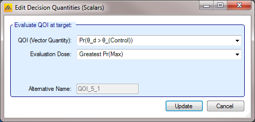
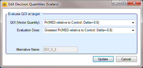
A decision QOI consists of (1) a QOI that has been calculated for each dose, and (2) a method of choosing a dose to use the QOI value of. Choosing the dose can be done either by using a target Dose QOI like Pr(Max), Pr(EDq…), etc, by choosing the dose with the highest or lowest value of a QOI, or by explicitly choosing a dose level in advance.
As an example using a target QOI, you can imagine evaluating a decision QOI that is specified to choose the probability of being better than Control by 2 units Pr(\(\theta_d - \theta_0 > 2\)) based on the arm with the highest ED90 EDq relative to control; Quantile 0.9.
Instead of a Target Dose QOI, it is also possible to specify a specific dose, or to use the terms “Max probability over all doses” and “Min probability over all doses” which mean that the dose with the minimum or maximum value of the per dose QOI is used. This enables:
Decisions QOIs testing specific doses, for example by defining a Posterior probability QOI that compares all doses against the lowest dose, and then a Decision QOI using that posterior probability with the highest dose selected as the target dose it is possible to based decisions on the posterior probability that the highest dose is better than the lowest dose.
A Decision QOI using “Max probability over all doses” allows a decision to be based on whether a probability or p-value is greater than a threshold at any dose, or less than a threshold at all doses.
A Decision QOI using “Min probability over all doses” allows a decision to be based on whether a probability or p-value is less than a threshold for any dose or greater than a threshold at all doses.
There is one special case: if the QOI chosen is the Trend Test p-value, then because this is not actually a per-dose value, only one “Target dose” can be selected: “Overall Significance”.
Standard Evaluation Variables
These 2 parameters are used across some of the default QOIs and hence specified outside the normal QOI dialog boxes.
The CSD value
and whether absolute or relative to the Control arm
these are used in both the default “Pr(CSD)” and the “MED relative to Control” QOIs.

Note that the CSD value here is designed to be usually entered as a positive value, as in earlier versions of FACTS. Its sign is automatically adjusted if “lower score means subject improvement” or if the trial is a non-inferiority trial.
These adjustments are not made for other user entered QOIs. The directions of comparison both for the definition of the probability to be calculated and the comparison of the resulting probability with a threshold are under the user’s control, as are whether delta’s are negative or positive. This allows the user to define QOIs in whatever fashion is natural to them and their team.
The direction of comparison for default QOIs
Note that as a result of being able to specify whether a higher or lower response represents improvement, and whether the aim is superiority or non-inferiority, the CSD or the NIM must always be a positive value. FACTS will automatically determine which direction is appropriate (e.g. if lower values are subject improvement, the engine will realize a CSD will need to be subtracted from the control score before comparing with the estimate of response on a treatment arm).