Accrual
The Accrual sub-tab provides an interface for specifying accrual profiles. Accrual profiles define the mean recruitment rate week by week during the course of the trial. Virtual subjects are simulated from a Poisson process in which the expected number of subjects per week is allowed to change week by week.
Accrual profiles are shown as a list on the left of the screen, as depicted below. These accrual profiles may be renamed by double-clicking on them and typing a new profile name. After creating a profile, the user must create at least one recruitment region. Early in the trial design process, detailed simulation of the expected accrual pattern is typically not necessary and a single region with a simple mean accrual rate is sufficient.
To model the expected accrual rates more precisely over the course of the trial, the user may specify multiple regions for each accrual profile and separately parameterize them. Regions are added via the table in the center of the screen Figure 1. Within this table, the user may modify:
the peak mean weekly recruitment rate,
the start date (in weeks from the start of the trial) for this recruitment region,
whether the region will have a ramp up phase and if so when the ramp up will be complete (in weeks from the start of the trial).
Whether the region will have a ramp down, and if so when the ramp down start and when the ramp down will complete (in weeks from the start of the trial).
Ramp up/ramp down define simple linear increase/decreases in mean recruitment rate from the start to the end of the ramp. Note that simulation of accrual is probabilistic, but ramp downs are defined in terms of time, so even if ramp downs are planned so that at the average accrual rate they will occur as the trial reaches cap, there is a risk in simulations when accrual has been slower than average, that ramp downs occur before the full sample size is reached. It is advisable to have at least one region that doesn’t ramp down to prevent simulations being unable to complete.
A graph of the recruitment rate of the highlighted region is shown as well. As the recruitment parameters are changed, the graph will update to show the time at which full accrual is reached. An accrual profile that does not reach full accrual is invalid and cannot be used to run simulations.
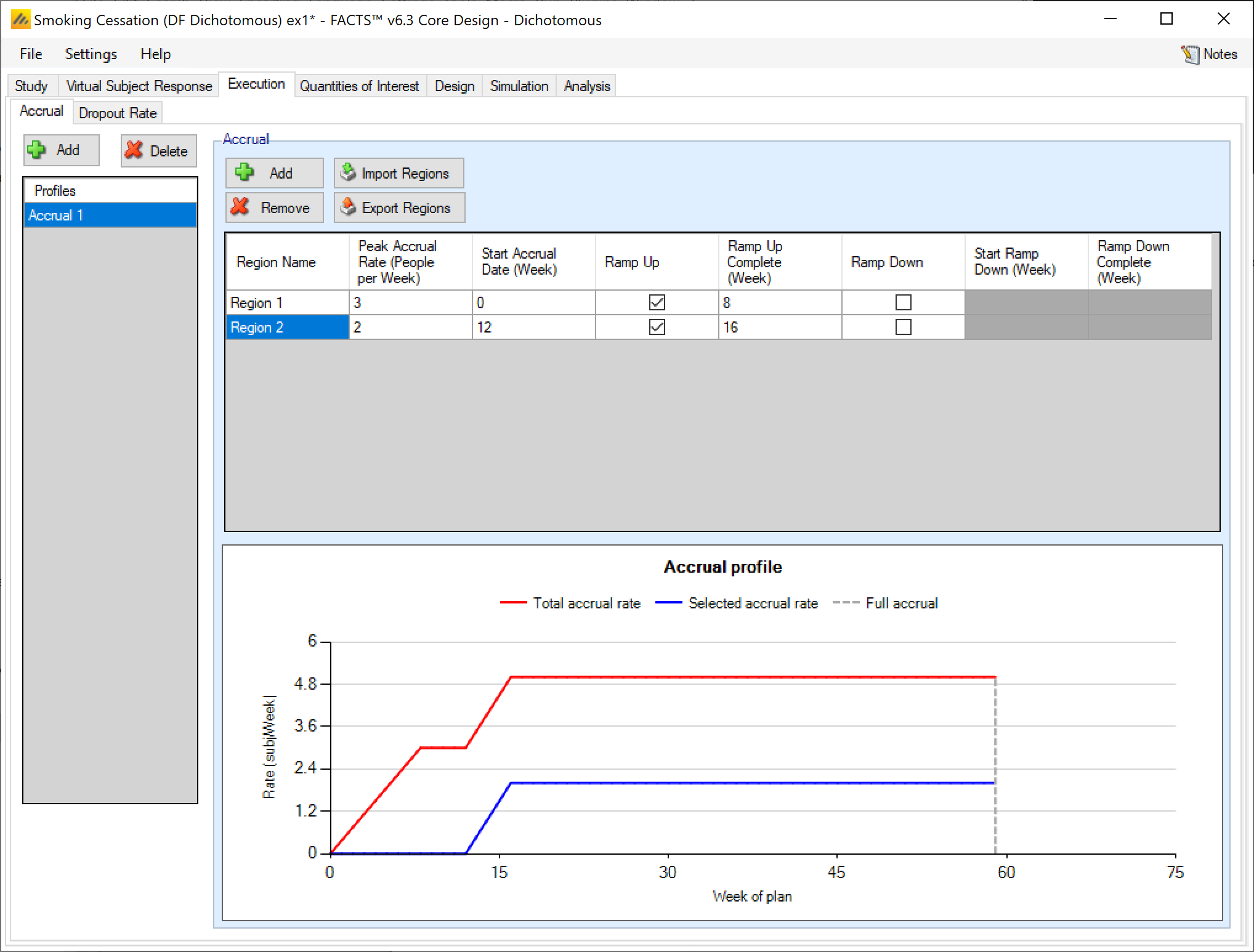
In the screenshot above you can see the two step ramp up in accrual from two regions – each starting at different offsets into the trial.
Note that the accrual profile graph is only the mean expectation; actual accrual is simulated using exponential distributions for the intervals between subjects, derived from the mean accrual profile specified here. Thus some simulated trials will recruit more quickly than this and some more slowly.
There are commands to import and export region details from/to simple external XML files. When importing, the regions defined in the external file are added to the regions already defined, they don’t replace them.
This is an example of a very simple region file defining just one region:
<?xml version="1.0" encoding="utf-8"?>
<regions>
<region>
<name>Region 1</name>
<rate>5</rate>
<start>0</start>
<ramp-up />
<ramp-down />
</region>
</regions>
Deterministic Accrual
If “Deterministic” accrual has been specified on the Study > Study Info tab, then on the Accrual tab, rather that specifying an accrual profile from which subject recruitment times are simulated, the user loads a file of specific accrual dates for every subject.
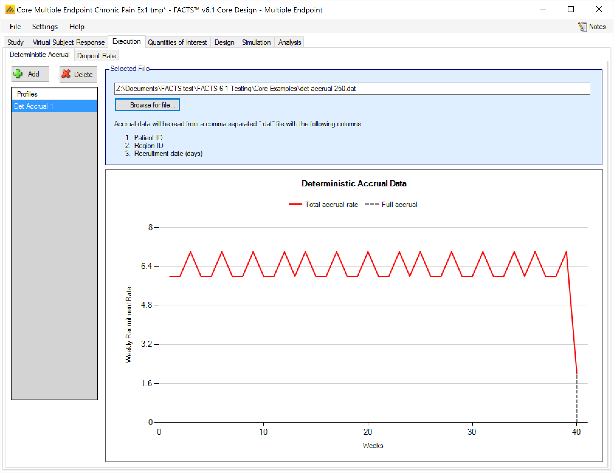
The user specifies a “.dat” file to load that contains the subject accrual dates in weeks This value is in weeks from FACTS 7.0 onwards, previously it was in days. from the start of the trial.
The required file format is a text file with comma separate values. One row per subject, with 3 fields on each row:
the subject ID, (an integer)
the ID of the region where the subject was recruited (an integer)
and the subjects randomization date (in weeks from the start of the trial – this is a ‘real’ number allowing fractions of a week to be specified)
The file must contain sufficient entries to allow the maximum number of subjects specified on the Study > Study Info tab to be recruited.
After successfully loading a file, the FACTS GUI shows a plot of the resulting weekly accrual rate
Drop-out Rates
The Dropout Rate sub-tab provides an interface for specifying dropout profiles; these define the probability of subjects dropping out during the trial.
Dropout profiles are listed on the left of the screen, as depicted below. These profiles may be renamed by double-clicking on them, and typing a new profile name. The default dropout scenario is that no subjects drop out of the study before observing their final endpoint data.
The continuous, dichotomous, and multiple endpoint engines allow specification of dropout rate slightly differently than the time-to-event engine.
For the continuous, dichotomous, and multiple endpoint engines, if dropouts are expected, the user can specify either “Dropouts per Dose,” or “Dropouts per Dose per Visit,” to specify a non-zero dropout rate.
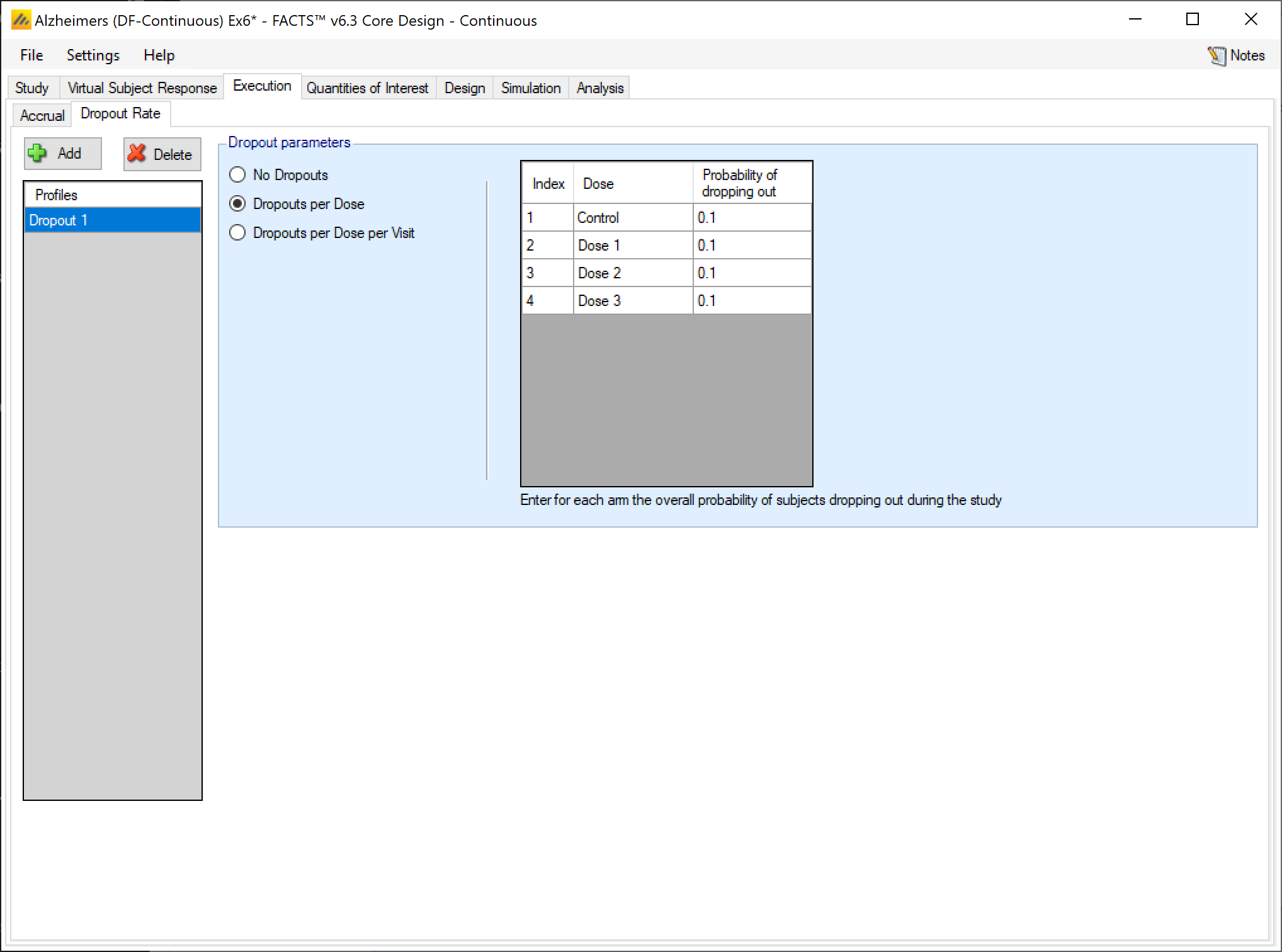
If “Dropouts per Dose” is selected, then each subject has a probability of not having an observable final endpoint value equal to the dropout rate of the dose that subject is randomized to. If each subject has multiple visits and “Dropouts per Dose” is selected, then the conditional probability of dropping out before each visit given that the subject had not dropped out up to the visit before rates are all equal. In other words, if the total dropout rate is \(\pi_D\), the probability of dropping out between visits \(i\) and \(i+1\) given that the subject had not dropped out at visit \(i\) is \(1 - \left( 1 - \pi_{D} \right)^{\frac{1}{V}}\) where \(V\) is the total number of visits.
If “Dropouts per Dose per Visit” is selected, then each subject has a user specified probability of dropping out before a visit \(v\) that is specified as the conditional probability of dropping out before visit \(v\) given that that they had not dropped out by visit \(v-1\). This leads to a total dropout rate \(\pi_D\) for a participant that is equal to:
\[\pi_{D} = 1 - \prod_{v = 1}^{V}{(1 - \pi_{v})}\]
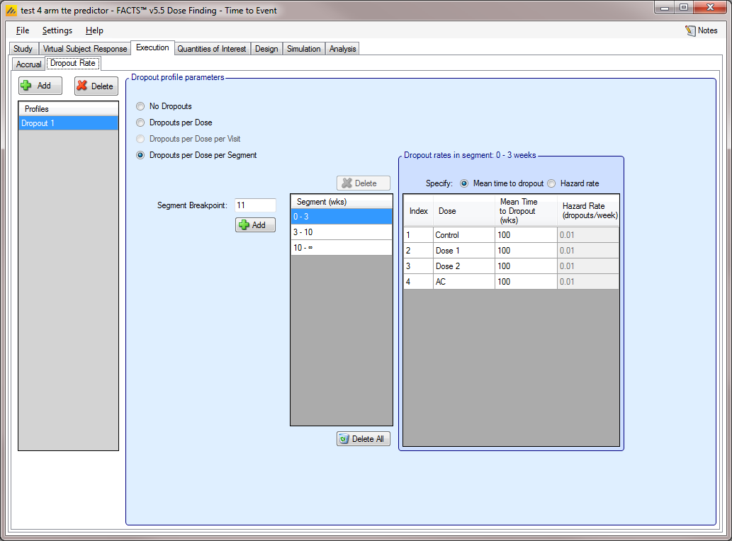
For time-to-event trials, the dropout scenario is one of:
No dropouts included in the simulation (“No Dropouts”);
Specifying “Dropouts per Dose”
Specifying “Dropouts per Dose per Visit” (only if visits are used)
Specifying “Dropouts per Dose per Segment”
In any of the above non-zero dropout rate scenarios, the dropout rates can be specified either by the mean time or hazard rate (in weeks) of an assumed exponential time to dropout. When specifying the “Dropouts per Dose,” the hazard rate for simulating dropouts is constant over time, but varies by dose.
When specifying “Dropouts per Dose per Visit,” the probability of dropping out between visits (not the hazard rate) is specified for each visit. This is the same way that dropouts are specified for continuous and dichotomous trials. Additionally, the post-final visit dropout rate is specified as a hazard rate moving forward. If the subject does not drop out before the final visit they have an exponentially simulated dropout time after that final visit.
Finally, the “Dropouts per Dose per Segment” option allows for a set of dropout specific time segments to be entered. These segments do not have to match the segments used in defining the control hazard rate (or segments used in the design). The dropout hazard rate is individually specified per arm and segment, and dropout times are piecewise exponential using those pieces.
In the time-to-event engine every subject has a latent simulated dropout time. This dropout time will only be “known” in the simulated trial if the subject accrues enough exposure to observe the dropout and the subject does not experience a primary endpoint event before the dropout time is reached.
Similarly, if a subject drops out of the study before they would have observed a predictor endpoint or a primary analysis event, then that event is never known to the simulation because the subject’s follow-up is truncated at dropout time.