LOCF (Last Observation Carried Forward)

The simplest possible longitudinal model. If {$y_{it}$} is the set of observed responses from early visits, and $y_{i t_m}$ is the last observed value of $y_{i t}$, then the LOCF model for the final endpoint $Y_i$ is

\[Y_i\mid \{y_{it}\} = y_{it_m}\]

In the continuous engine $t_m$ can be any earlier observed visit including the baseline value.

Linear Regression

Shiny App

The following shiny application for a tool that helps visualize and set priors for the linear regression longitudinal model.

See here.

The linear regression model fits a simple linear model from the data at each visit with the final visit

\[Y_i \mid y_{it} \sim \alpha_t + \beta_t y_{it} + \text{N}(0,\lambda_t^2)\]

The parameter $\alpha_t$ is the intercept of the model for visit t, and the parameter $\beta_t$ is a multiplicative modifier (slope) of the response observed longitudinal at visit $t$ to adjust the prediction of the final endpoint.

Imputation of the final endpoint value for a subject using the linear regression longitudinal model is based on only the latest observed visit’s endpoint value.

The default setting of “Same priors across all model instances and visits,” implies that each parameter $\alpha$, β, and λ have the same prior for all t. Estimation of those parameters is still done independently for each model instance. The one prior across all model instance are formulated as:

\[\alpha_t \sim \text{N}(\alpha_\mu, \alpha_\sigma^2)\] \[\beta_t \sim \text{N}(\beta_\mu, \beta_\sigma^2)\] \[\lambda_{t}^{2} \sim \text{IG}\left( \frac{\lambda_{n}}{2},\frac{\lambda_{\mu}^{2}\lambda_{n}}{2} \right)\]

The above prior formulation may not be desirable if specifying priors that are not extremely diffuse – especially on the $\beta$ parameters. Instead, selecting “Specify priors per visit across all model instances,” will share the prior specification across all instances of the model, but allows for different priors to be put on the parameters associated with each visit. The user inputted prior parameters are now subscripted with $t$ to denote the visit they correspond to. These priors apply to all model instances:

\[\alpha_t \sim \text{N}(\alpha_{\mu_t}, \alpha_{\sigma_t}^2)\] \[\beta_t \sim \text{N}(\beta_{\mu_t}, \beta_{\sigma_t}^2)\] \[\lambda_{t}^{2} \sim \text{IG}\left( \frac{\lambda_{n_t}}{2},\frac{\lambda_{\mu_t}^{2}\lambda_{n_t}}{2} \right)\]

It is also possible to specify priors “Per model instance and visit,” in which every visit has separate priors, and those differing priors vary across model instances. This is the most flexible prior specification method. The user inputted prior parameters are now subscripted by both t for visit and i for model instance.

\[\alpha_{ti} \sim \text{N}(\alpha_{\mu_{ti}}, \alpha_{\sigma_{ti}}^2)\] \[\beta_{ti} \sim \text{N}(\beta_{\mu_{ti}}, \beta_{\sigma_{ti}}^2)\] \[\lambda_{ti}^{2} \sim \text{IG}\left( \frac{\lambda_{n_{ti}}}{2},\frac{\lambda_{\mu_{ti}}^{2}\lambda_{n_{ti}}}{2} \right)\]

A potential starting place for non-informative prior values would be

$\alpha$: mean of 0, SD $\ge$ largest expected response
$\beta$: mean of either 0 or $\frac{\text{final visit time}}{\text{early visit time}}$, SD $\ge$ largest expected ratio of final visit to first visit
$\lambda$: mean of expected SD of the endpoint (‘sigma’), weight of 1. The variability of the prediction from the longitudinal model (based on an observed intermediate response) should be less than that based solely on the treatment allocation, thus this is a weakly pessimistic prior on the effectiveness of the longitudinal model that should be quickly overwhelmed by the data.

This model is easy to understand and can be used even if there is only one visit, but doesn’t get more powerful if there are more visits. Its power will depend on the degree of correlation between the intermediate visit response and the final response.

Time Course Hierarchical

The Time Course Hierarchical models the relationship between subjects’ early responses and their final response. It incorporates a per-subject offset from the mean response and a scaling factor from each visit to the final endpoint, but with no model of the change from visit-to-visit.

The response at the $t_{th}$ visit for the $i^{th}$ subject, having been randomized to the $d^{th}$ dose is modeled as:

\[y_{it} \sim e^{\alpha_t}(\theta_d + \delta_i) + \text{N}(0, \lambda_t^2)\]

The imputed final response (visit $T$$) for the $i^{th}$ subject, having been randomized to the $d^{th}$ dose is modeled as:

\[Y_{iT} \sim \theta_d + \delta_i + \text{N}(0, \lambda_T^2)\]

(i.e. $\alpha_T$ is 0).

The model parameters can be interpreted as follows:

$\theta_d$: the estimated mean response at the final visit in dose $d$ from the dose response model.
$\delta_i$: the estimated patient level random effect around the mean final response ($\theta_d$) for the dose $d$ that patient $i$ is randomized to.
$\alpha_t$: a scaling parameter that determines the proportion of the final response that is observable at visit $t$. A value of $\alpha_t=0$ indicates that the expected value of early visit $t$ is equal to the estimated final visit mean $\theta_d$. A value of $\alpha_t= −0.69315$ indicates that the expected value of early visit $t$ is 50% of the estimated final visit mean $\theta_d$.
$\lambda_t^2$: the variance of the endpoint around the estimated mean response at visit $t$.

The prior for $\alpha_t$ is a normal distribution with a user specified the mean and standard deviation:

\[\alpha_t \sim \text{N}(\alpha_\mu, \alpha_\sigma^2)\]

The prior for the $\delta_i$ terms is a normal distribution with a mean of 0 and variance τ².

\[\delta_i \sim \text{N}(0, \tau^2)\]

$\tau^2$ is estimated as part of the longitudinal model, and has an inverse gamma prior distribution with prior central value $\tau_\mu$ and weight (in terms of “equivalent number of observations”) $\tau_n$:

\[\tau^{2} \sim \text{IG}\left( \frac{\tau_{n}}{2},\\\frac{\tau_{\mu}^{2}\tau_{n}}{2} \right)\]

The prior for the $\lambda_t^2$ terms is an inverse gamma distribution with prior central value $\lambda_\mu$ and weight (in terms of “equivalent number of observations”) $\lambda_n$:

\[\lambda_{t}^{2}\sim\text{IG}\left( \frac{\lambda_{n}}{2},\frac{\lambda_{\mu}^{2}\lambda_{n}}{2} \right)\]

A reasonable starting place for prior values would be

$\alpha_t$: mean of -2, SD of 2, … so the prior ~70% interval for $\alpha_t$ is between -4 and 0 (+/1 1 SD) and thus the prior 70% interval for $e^{\alpha_t}$ to be between 0.02 and 1.
$\tau$: mean set to the expected SD of the endpoint (‘sigma’), with a weight of 1.
$\lambda_t$: mean set to the expected SD of the endpoint (‘sigma’), with weight of 1.

We would expect $\tau^2 + \lambda^2 \approx \sigma^2$, thus to specify a prior mean of $\sigma$ for each with a weight of 1 is a weakly pessimistic prior that should be quickly overwhelmed by the data.

This model is useful if there is thought to be a significant per-subject component to the response that should be manifest at the intermediate visits, and sufficient visits for the per-subject component to be estimated.

Kernel Density

The Kernel Density Model longitudinal model is a non-parametric re-sampling approach that is ideal for circumstances where the relationship between the interim time and the final endpoint is not known or not canonical.

The procedure is as follows. Assume an interim value for patient $i$ at time $t$, $Y_{it}$. Patient $i$ does not have an observed final endpoint at time $T$, so one is to be imputed. Let $(X_{1t},X_{1T}), \ldots, (X_{nt}, X_{nT})$ be the set of values for the previous subjects for whom there exists an interim value $X_{*t}$ and final value $X_{*T}$.

To impute a value of $Y_{iT}$ given $Y_{it}$, a pair $(X_{kt},X_{kT})$ is selected with probability based on the pair’s time $t$ visit response’s proximity to the observed $Y_{it}$:

\[\Pr\left(\text{Selecting}\left( X_{kt},\\X_{kT} \right) \right) = \frac{\exp\left( - \frac{1}{2h_{X_{t}}^{2}}\left( Y_{it} - X_{kt} \right)^{2} \right)}{\sum_{k = 1}^{n}{\exp\left( - \frac{1}{2h_{X_{t}}^{2}}\left( Y_{it} - X_{kt} \right)^{2} \right)}}\]

Then, a value of $Y_{iT}$ is imputed from the following distribution, which uses the selected pair’s final endpoint response $X_{kT}$:

\[Y_{iT} \sim \text{N}(X_{kT}, h_{X_T}^2)\]

The bandwidths $h_{X_t}$ and $h_{X_T}$ are selected based on the criterion given by Scott (1992). That is,

\[h_{X_{j}} = \sigma_{X_{j}} \left( 1 - \rho^{2} \right)^{\frac{5}{12}} \left( 1 + \frac{\rho^{2}}{2} \right)^{- \frac{1}{6}}{\\n}^{- \frac{1}{6}}\text{ for } j = t \text{ and } T\]

where $\sigma_{X_j}$ is the standard deviation of the observed responses at time $j$, $n$ is the number of pairs $(X_{*t},X_{*T})$ that were chosen between, and $\rho$ is the correlation coefficient between $X_t$ and $X_T$ in the pairs $(X_{1t},X_{1T}), \ldots, (X_{nt}, X_{nT})$.

The Kernel Density model does not take prior distributions as input. So long as each early visit has more subjects with an observed early response and final response than the value entered in “Minimum number of participants with an early visit and final visit needed to estimate kernel bandwidths for that early visit:” then this algorithm runs without regard for user input.

If any visit has fewer subjects with early data and final data than the specified minimum number of participants, then instead of calculating the values of $h_{X_t}$ or $h_{X_T}$ the input values of “Fixed kernel bandwidth $h_x$:” and “Fixed kernel bandwidth $h_y$:” are used.

For $h_x$ and $h_y$, possible starting values are the expected SD of the endpoint (‘sigma’). The default value for the minimum number of subjects with complete early and final visits is 6, but this value can be set to anything greater than 0 that the user desires.

The Kernel Density model is effective and flexible with no model assumptions, but its computational overhead is large. Simulations may take $\sim 10$ times longer to run, and having no prior model there has to be ‘in trial’ data before it can come into play.

ITP

The ITP (Integrated Two-component Prediction) model fits an observation for patient $i$ on dose $d$ at visit $t$ as:

\[y_{idt} = \left( \theta_{d} + s_{id} + \epsilon_{idt} \right)\left( \frac{1 - \text{exp}\left( kx_{idt} \right)}{1 - \text{exp}(kX)} \right)\]

where \[\epsilon_{idt} \sim \text{N}(0, \lambda^2)\] \[s_{id} \sim \text{N}(0, \tau^2)\]

and $\theta_d$ is the mean estimate of the final endpoint for dose d using all complete and partial data and assuming an independent dose response model on the doses. $s_{id}$ is a subject specific random effect, $k$ is a shape parameter, $x_{idt}$ is the time $y_{idt}$ is observed, $X$ is the time to final endpoint, and each $\epsilon_{idt}$ is a residual error.

The ITP model is similar to the Time Course Hierarchical above in that both models estimate subject specific component of the response. The biggest difference between the two is that in the ITP models the response changes over time as a parametric function based on the parameter $k$, rather than having a separately estimated $e^{\alpha_t}$ for each visit.

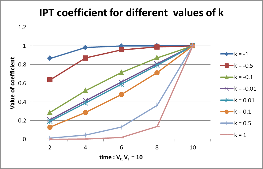
The shape parameter $k$ determines the rate at which the final endpoint’s eventual effect is observed during a subject’s follow-up. A value of $k=0$ indicates that the proportion of effect observed moves linearly with time. A value of $k<0$ means that the eventual final effect is observed earlier in follow-up and plateaus off as time moves towards the final endpoint. A value of $k>0$ indicates that less of the total final endpoint effect is observed early in follow up, but as time approaches the final endpoint time the proportion of the effect observed increases rapidly. Values of $k$ less than 0 tend to be more common than values of $k$ greater than 0. See the figure below for a visualization of the different response-over-time curves that can be estimated with the ITP model.

Figure 1: Examples of a variety of ITP models with the shape parameter k ranging from -1 to 1.

The priors for the parameters in the ITP model are: \[k \sim \text{N}(\mu_k, \sigma_k^2)\] \[\theta_d \sim \text{N}(\mu_{\theta_d}, \sigma_{\theta_d}^2)\] \[\tau^2 \sim \text{IG}\left( \frac{\tau_{n}}{2},\frac{\tau_{\mu}^{2}\tau_{n}}{2} \right)\] \[\lambda^2 \sim \text{IG}\left( \frac{\lambda_{n}}{2},\frac{\lambda_{\mu}^{2}\lambda_{n}}{2} \right)\]

A reasonable starting place for prior values would be:

$\theta_d$: mean of the expected mean improvement from baseline on the Control arm, with SD greater than or equal to the expected treatment effect size.
$k$: a mean of 0 and SD of 2, if subject improvement is expected to be rapid and then diminishing, the prior mean might be -0.5 or -1, if subject improvement is expected to be initially slow or non-existent then increasing, the prior mean might be 0.5 or 1.
$\tau$: mean set to the expected SD of the endpoint (“sigma”), with a weight of 1.
$\lambda$: mean set to the expected SD of the endpoint (“sigma”), with a weight of 1.

The ITP model implies that the variance of the observations shrinks towards 0 with the mean (so early visits have reduced expected responses and variances). The ITP model may result in biased estimates of $\theta_d$ and/or the variance terms $\tau^2$ and $\lambda^2$ if the mean-variance relationship assumed by the ITP model is not present in the observed data. If the model assumptions are correct this can be a very effective longitudinal model.