Introduction

Purpose of this document

This document describes how use the FACTS Dose Escalation (DE) CRM design engine. It is intended for all end users of the system.

Scope of this document

This document covers the FACTS Dose Escalation N-CRM design engine user interface.

This document does not address the internal workings of the design engines or algorithms, which are addressed in the associated Design Engine Specification. It also does not address the use of FACTS Core Designs or Enrichment Designs, which are covered in other User Guides.

The screenshots provided are specific to a particular installation and may not reflect the exact layout of the information seen by any particular user. They were taken from FACTS 6.3 and later installed on Windows 10. Different versions of Windows or the use of different Windows themes will introduce some differences in appearance. The contents of each tab, however, will be consistent with the software.

Citing FACTS

Please cite FACTS wherever applicable using this citation.

Definition of Terms

An overview of the acronyms and abbreviations used in this document can be found here.

FACTS Overview

This user guide assumes some limited general familiarity with FACTS and concentrates on describing the interface for designs using the N-CRM approach. See the FACTS Dose Escalation user guide for a general introduction to the FACTS Dose Escalation user interface.

The N-CRM is based on the method described in the paper (Neuenschwander, Branson, and Gsponer 2008). It is designed for use in oncology phase 1 trials, and we understand generally in use at Novartis for the majority of their trials of this type:

Dosing starts at a (very) low dose, strongly believed to be safe.
Usually after a cohort of subjects have completed their current dose, the dose to be used for the next cohort is selected. The selection of this dose is dictated by a combination of dose escalation rules, the estimate of the toxicity rate on the different doses and the target maximum tolerated toxicity, or toxicity band.
The endpoint per subject is binary: toxicity observed or not.
There is either a predefined set of doses to explore, or a dose range.
There is limited sample size.

FACTS 7.1 Changes to N-CRM

In FACTS 7.1 there were new features added to N-CRM:

It is now possible to backfill to the current escalation dose (also known as “frontfilling”).
It is now possible to specify a third queue concept – maximum number of patients in their DLT period on the current MTD estimate.
It is now possible to define the concept of “near” target/MTD as part of stopping rules, for both fine-grained and regular dosing.

FACTS 7.0 Changes to N-CRM

In FACTS 7.0 the only change was on the Analysis tab, when entering subject data manually, the FACTS GUI now ensures that a cohort number is entered for every subject.

FACTS 6.5 Changes to N-CRM

In FACTS 6.5 there was a new feature added to N-CRM:

It is now possible to generate a design report – a Word document describing design - once the design has been simulated. In FACTS 6.5 there was two small changes to the functionality:
When deriving toxicity/efficacy priors from quantiles at the lowest and highest doses, the “middle” probability option now refers to the median dose rather than the reference dose and is now optional. When pre-6.5 FACTS files are loaded in FACTS 6.5, the “middle” probability option will be ignored and replaced by 0.5.
When deriving toxicity/efficacy priors from specific quantiles the specification of at least two dose levels is now required whereas previously the specification of at least three dose levels was required.

In FACTS 6.5 there were some improvements in the simulated behavior:

Designs which include efficacy, the “Maximum cohorts used to determine MTD” parameter on the Allocation Rule tab is now observed, in FACTS 6.4 and earlier it was ignored.
In N-CRM designs using open enrollment without accrual pausing, FACTS will now output entries in the cohort file for subjects that have been lost following stopping rules being met.
In N-CRM designs using open enrollment, FACTS will no longer prematurely apply stopping conditions when there are still subjects whose outcomes have been observed, but not yet processed.
In N-CRM designs using open enrollment, FACTS will now report the selected MTD/MED/OSD and associated state to be the dose where the stopping conditions were first met, unless the MTD has subsequently decreased post stopping rules being met. This is to prevent a dose above the one selected when the stopping conditions were met being reported as the MTD when it is very likely that there is insufficient data on this higher dose to justify its selection. If rather than reporting the MTD at the point when the stopping rules where met, you would like the trial to resume if the dose selected as MTD has changed (and this the stopping rules possibly no longer met), ensure that the ”Pause accrual and wait for completers” option is selected on the “Stopping Criteria” tab. This allows the trial to resume if the recruitment cap has not been met.
FACTS Command Line mode and FLFLL (FACTS Linux File Loader Lite) now correctly handle the processing of N-CRM designs whose prior was derived using the “Legacy Prior” option.

FACTS 6.4 Changes to N-CRM

In FACTS 6.4 there were no changes to the Dose Escalation simulators.

FACTS 6.3 Changes to N-CRM

In FACTS 6.3 a number of changes were made to improve facilities in N-CRM, or improve the way existing facilities were implemented. These were:

New run-in options: the existing run-in scheme is available as “simple run-in”, “custom run-in” allows a specific sequence of doses and number of subjects to test at each dose to be specified, “small cohort pre-escalation” allows a run that uses a smaller cohort size but follows the dose escalation rules and over dose control.
New “backfill” options in open enrolment. Backfill allows subjects that become available at a time when they can’t be allocated to the current dose (because the maximum number of subjects without final results have already been allocated to the current dose).
Improved handling of “maximum subjects without final results” in open enrolment. In earlier versions of FACTS this was a “global” maximum, which led to a suboptimal allocation pattern and overly cautious rejection of subjects that became available. The new model applies a maximum “per dose” so that once the trial has escalated to a new dose strength, any subjects without final results on lower doses do not block allocation to the new dose, in addition it is possible to specify two different maximums – one for when a dose has just been escalated to but has not been “cleared” (typically smaller and more cautious), and one when a dose has been cleared but we continue to allocate to it because it is the target dose (typically larger and more confident). This method is such an improvement that we recommend moving any design using open enrolment to this new version of FACTS.
Improved Ordinal Toxicity model – the way the likelihood is calculated has been improved – reducing the uncertainty in the model fit. Any design using an ordinal model will need to re-calibrate the prior if you move the design to FACTS 6.3. If you have a design already complete, or in execution we recommend you remain using the earlier version of FACTS for that trial.

FACTS 6.2 Changes to N-CRM

In FACTS 6.2 features available separately in the other FACTS CRM engines (CRM (Toxicity), bCRM & CRM Ordinal) were all incorporated into N-CRM. This allowed these features to be used in conjunction with N-CRM’s target toxicity band methodology, overdose control and open enrollment features, as well as in conjunction with each other for the first time.

The new features are:

From CRM (Toxicity) the option to specify that the data is coming from ‘two groups’ and for the toxicity experienced in the two groups to be modelled with a joint model [CRM 2 Sample]. This allows a trial where there are two patient populations (such as adults and children) or where there are two versions of the treatment to be simulated.
From bCRM the option to model a second binary efficacy endpoint [bCRM] and the for dose allocation to proceed in two stages – the first to establish an MTD and the second to establish an MED.
From CRM Ordinal the option for the toxicity endpoint to be modelled not as binary endpoint, but one with different categories of toxicity, and with a joint model applied to the different categories [CRM Ordinal]. The endpoint can be to model either 3 or 4 categories of toxicity:
1. category 1 is “no toxicity”,
2. category 2 is “mild toxicity”,
3. category 3 is “toxicity”
4. category 4 (if included) is “severe toxicity”

All decision making is made in terms of the probability of observing a category 3 (or worse) toxicity.

FACTS 6.1 Changes to N-CRM

In FACTS 6.1 N-CRM has the new feature of ‘design variants’ that allow the user to easily simulate and evaluate an N-CRM design at different sample sizes. This change includes 4 elements:

Under the ‘Study’ tab the user can now specify the number of design variants, and for each variant the maximum study size in Cohorts.
On the simulation tab FACTS will display a copy of each simulation scenario for each variant.
The simulation results now include the Ppn of trials that stopped for each stopping reason: stopping because all doses are too toxic (the toxicity estimates exceed the overdose criteria), because a stopping rule was met or because the study cap was reached.
There are now a set of cross variant graphs that show trellis plots of the key summary graphs by design variant and scenario.

N-CRM Dose Escalation Design Concepts

In an N-CRM dose escalation trial, subjects are exposed to the novel treatment at increasing dose strengths, not progressing to the next dose strength until lower doses have been shown to be sufficiently safe, and not progressing beyond the dose which appears to display the maximum tolerated rate of toxicity, or the target rate of toxicity, the “Maximum Tolerated Dose” (MTD). To limit the risk of exposing subjects to a new, higher dose strength, subjects are allocated in “cohorts’ of a given size and no further subjects are recruited until all the subjects in the cohort complete treatment and follow-up. To enroll subjects quicker and introduce further options to manage the risk of exposure at new doses, FACTS allows “Open Enrolment” of new subjects, which is a form of design that dispenses with cohorts and is described in this section.

Once all the subjects in a cohort have completed, FACTS updates its analysis of the dose toxicity, re-evaluates the dose-escalation rules and selects the dose the next cohort will be allocated to. As well as the final results of each simulated trial, each time a cohort completes FACTS outputs the data available and the results of the analysis. These are referred to as “cohorts files”, and when you run the simulations, you can specify for how many of them you want these additional files written out.

The design’s default behavior is to allocate the next cohort to the model estimated MTD, but this is typically modified by several user specified rules. Note that if all the rules are met, the allocation is to the model estimated MTD, it will never allocate above it.

The rules that are available to modify this behavior, to achieve “not progressing to the next dose strength until lower doses have been shown to be sufficiently safe” are:

Starting dose: the dose strength to be allocated to the first cohort. (Specified on the Design > Allocation Rule tab)
Overdose control: a limit can be specified on the probability that a dose’s toxicity rate is above a certain level, and any dose for which this is true is excluded from allocation. (Specified on the Study > Toxicity tab)
Dose escalation rules: The size of the increase in dose strength from one cohort to the next can be specified (Specified on the Design > Allocation Rule tab).
Single patient / small cohort run-in: a fixed dose allocation scheme can be specified, using a different (typically smaller) cohort size. That is applied without reference to any other rules or to the results of the analysis as long as no toxicities have been observed. If the trial includes what is thought to be a number of weak doses that are likely to have toxicity below the target rate, but are still required to be tested, using a run-in can make testing these doses cheaper and quicker.

In the sections to follow, we describe overdose control, dose escalation rules and run-in features in the conventional context of cohort enrolment and a limited number of possible doses. We also describe the options FACTS allows to model the subjects in the trial as belonging to 2 different groups and the options to simultaneously model an efficacy endpoint. We subsequently describe how these are modified if:

there are many potential dose strengths in a certain range that could be, but don’t have to be, administered in the trial (“fine grain dosing”).
we choose not to limit enrolment to cohorts but enroll subjects continuously (“open enrolment”).

Overdose Control

Overdose control can be specified on the Study > Toxicity tab. Overdose control specifies a limit on the probability that a dose has a toxicity rate above a certain level. After fitting the Bayesian logistic regression model, all doses for which the posterior probability that their toxicity rate lies above the specified level exceeds the specified limit are ineligible for allocation. Because the Bayesian Logistic regression is monotonic, this means that after every analysis either all doses are permitted for allocation or there will be a dose level above which no dose is permitted for allocation.

The overdose control is specified in terms of the “toxicity bands” (concept of allowing ranges for the target toxicity, excess toxicity, unacceptable toxicity and under-dosing explained in more detail in this section) and can either be in terms of the “excess and unacceptable toxicity bands” or just the “unacceptable toxicity band”. The “excess and unacceptable toxicity band” is every toxicity rate above the upper bound of the target band. Care should be taken when setting the permitted threshold for this joint band. If set below 0.5, it will likely exclude doses whose mean expected toxicity rate is within the target band with the risk that this makes the escalation decision in the design too cautious. Initially it might be recommended to just use the “unacceptable band” for specifying the overdose control. This allows an overdose control that is more strict – for example: “exclude any dose where the probability that the toxicity rate is above 0.6, is greater than 20%“. The lower bound for the unacceptable band can be set wherever desired, its only role is in defining this band for overdose control. It is also possible to specify that the limit changes over the course of the trial, allowing the overdose control to become stricter as more information becomes available. For example, one could reduce the permitted probability of a dose having a toxicity rate in the unacceptable band from 50% to 25% in steps of 2.5% after every cohort.

Dose Escalation Rules

The dose escalation could be solely controlled by the overdose control (as originally proposed in (Neuenschwander, Branson, and Gsponer 2008)), however this means that the escalation behavior is very dependent on the interplay between the prior and the observed data. Usually, teams prefer to have a fixed set of rules in place ensuring the escalation behavior is sufficiently cautious. FACTS has an option to just use overdose control or to use a combination of overdose control and a set of fixed escalation rules. In the latter case, the following rules can be set in the Design > Allocation Rule > Allocation tab:

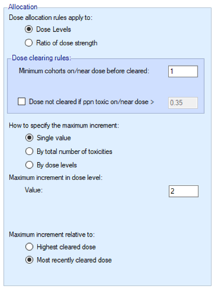
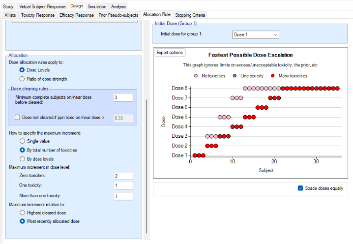
We introduce the notion of whether a dose has been “cleared”. A dose is cleared once we have sufficient data on it (usually, but not necessarily, the results of one cohort, but if the cohort size is small, for example 2 subjects, perhaps more than one cohort will be required). This can be supplemented by a rule that if the observed raw toxicity rate at the dose exceeds a certain limit, then the dose is not counted as cleared (this rule is usually unnecessary if overdose control limits have been set). Once a dose has been cleared, it stays cleared, meaning there is “maximum cleared dose”. The number of dose increments or the factor of dose strength above the current cleared dose that can be allocated to is then specified. For example, with doses of 12.5, 25, 50, 100, 150, 200, 250, we might allow escalation at two dose increments a time. In the figure below, you see the combination of settings used to achieve this behaviour alongside the “Fastest Possible Dose Escalation” plot on the right:

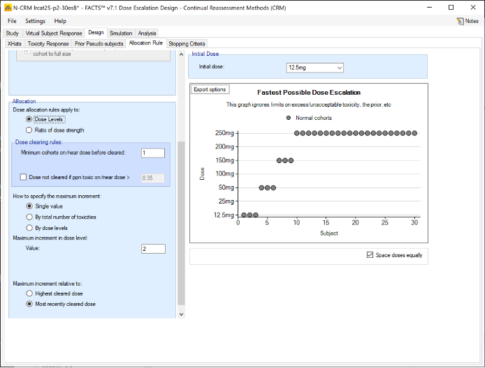
Figure 3: Escalation by number of dose increments

Alternatively, we can specify the permitted escalation as a ratio, for example we might allow the dose strength to be at most tripled at each escalation, which, with the example dose strengths, makes the initial escalation more cautious:

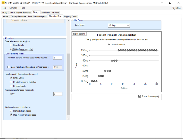
Figure 4: Escalation by dose strength factor

The escalation rules can be adjusted so that instead of a single increment rule, there are different increments depending on the dose, or depending on the number of observed toxicities. To modify our earlier example, we can allow escalation by 2 dose levels while no toxicities have been observed, but limit it to only one dose level once one or more toxicities have been observed:

Figure 5: Escalation increment varying by number of toxicities

Lastly escalation can be relative to the highest cleared dose, or relative to the last dose allocated.

To summarize the allocation procedure:

The current maximum cleared dose is identified.
The current data is analyzed using the Bayesian Logistic Regression model.
The overdose rules are evaluated and all doses exceeding the overdose control limit are excluded from this escalation selection.
From the remaining doses, the dose best meeting the target MTD or target toxicity interval objective based on the model is selected as the “target dose” (TD).
If the TD is at or below the current maximum cleared dose, the next cohort is allocated to the TD.
If the TD is within the escalation rules of the current maximum cleared dose, the next cohort is allocated to the TD.
Otherwise, the next cohort is allocated to the highest dose above the current maximum cleared dose as allowed by the escalation rules.

Initial Run-in

The purpose of defining a run-in is to define a fixed allocation behavior to be followed up to the first toxicity being observed. The specified number of subjects to allocate to each dose in the run-in and which doses to test are specified. This scheme is followed until a toxicity is observed or we reach the end of this fixed scheme.

Three forms of run-in specification are available:

Simple: allocates a small cohort to every defined dose in ascending order (unless fine grain doses - see this section – have been specified, in which case the escalation rules are followed).
Custom: allocates a defined number of subjects (possibly varying by dose) to selected doses in ascending order.
Small cohort pre-escalation: allocates a small cohort, but follows the escalation rules assuming just a single small cohort is required to clear a dose.

All run-in schemes can be modified in a number of ways:

Specifying a maximum dose at which the run-in stops if no toxicities are observed until that dose.
If ordinal toxicities are being simulated, the run-in may should at the first observed category 2 toxicity (rather than a category 3 toxicity)
Whether the subjects used in the run-in should be counted towards the trial sample size or not.
When a toxicity is observed the standard behavior is to allocate to the minimum of: the last dose tested in the run-in, the current TD or the highest dose that can be allocated to by the overdose rules. This can be replaced by expanding the allocation on the current dose to make it a full cohort as specified in Study > Study Info tab (this option is particularly useful in conjunction with stopping for a category 2 toxicity).

Two Groups

FACTS has the option to model the subjects in the trial as belonging to two different groups, these can be either:

Two groups distinguished by a baseline property of the subjects, for example adults and paediatrics.
Two groups separated by a difference in treatment (and selected randomly), for example the study drug alone or in combination with an additional drug.

There are options for when group 2 starts enrolling:

They can be recruited sequentially – group 1 then group 2.
They can be recruited in parallel
The second group can be started when the allocation to the first group reaches a particular dose
The second group can be started when the number of subjects allocated to group 1 reaches a particular threshold.

A joint model is fitted to the two groups.

The first group is modeled:

\[ logit(p_{1j}) = \alpha + \beta \hat{x}_j \]

The second group is modeled:

\[ logit(p_{2j}) = (\alpha + a) + (\beta + b) \hat{x}_j \] With separate priors and some optional constraints on \(a\) and \(b\). Dose escalation and stopping are judged independently for the two groups.

Efficacy

FACTS has the option to additionally model an efficacy endpoint. There are currently two limitations in simulation:

Only a binary efficacy endpoint can be simulated
The efficacy endpoint is assumed to be available at the same time as the toxicity endpoint.

The efficacy and toxicity endpoints are modelled separately. There are options to specify early stopping rules for finding the MTD, and to specify a cap on the sample size that can be spent finding the MTD. Once these rules are met, then allocation is towards the Minimum Efficacious Dose (MED) – if this is below the MTD. If the estimated MED lies at or above the estimated MTD, the allocation is at the estimated MTD.

If while allocating to the estimated MED further toxicity results change the estimate of the MTD, and if there is now insufficient information on the MTD as specified by the early stopping rules for finding the MTD, allocation switches back to allocating to the estimated MTD, if the sample size cap for finding the MTD allows.

Fine Grain Dosing

In some settings, e.g. when the drug is delivered in solution by IV or when manufacturing allows any dose in a range from say 100mg to 400mg in steps of 10mg, dose strengths need not be restricted to just a small number of pre-defined levels. FACTS has a feature that allows this to be simulated, not with a continuous range of doses, but with “fine grain” dosing.

FACTS supports the specification of a range of doses from a minimum to a maximum with doses either equally spaced or spaced with equal ratio. Using dose ratio makes most sense it you want to use the dose strength whilst believing the effect will be roughly log-dose. Using dose ratios, it’s necessary to accept FACTS reporting dose strengths only close to those desired. As an example, if the main doses followed a dose doubling scheme: 12.5, 25, 50, etc., one might use fine grain dosing with dose space ratios of approximately the 4th root of 2 (1.1892). The resulting doses are 12.5, 14.865, 17.677, 21.022, 24.999, 29.729, 35.354, 42.043, 49.998, etc., which means there are three dose levels between each of the original doses.

There are two alternatives:

Use nominal dose strengths 1, 2, 3, 4, … (i.e. assuming the dose spacing is linear in expected effect) and label the doses according to their actual strength.
Use a fixed dose interval (e.g. 12.5 resulting in doses of 12.5, 25, 37.5, 50, 62.5, etc.) so the lower doses (of the original scheme) have fewer (or no) intermediate doses and the higher doses have many more. The dose escalation rules can be specified in terms of dose strength ratio to achieve the required escalation, for example allowing dose escalation with a dose strength ratio of 2 will result in the initial escalation using doses 12.5, 25, 50, 100, etc.

As well as possibly adjusting the dose escalation step size to accommodate the new dose levels on the Design > Allocation Rule tab, there are two other rules that may need modification:

To count a dose as “cleared”, we might now count cohorts on nearby doses to count towards the required clearing total. This is specified as the “Max ratio of dose strengths considered as near” (if dose allocation rules apply to ratio of dose strength) or “Delta in dose strength considered as near” (if dose allocation rules apply to dose strength) on the Design > Allocation Rule tab.
- For example, if we have doses at roughly 4th root of 2 intervals, we might count any dose within a ratio of 1.2 as “near” so that any cohorts allocated to immediate neighbor doses count towards clearing a dose.
- Alternatively, if we have doses every 12.5mg from 12.5 to 400, counting any dose within a ratio of 1.1 will mean that from dose 125 and above, immediate neighbor doses (within 12.5) count towards clearing a dose, and from dose 250 and above, doses within 25mg (two immediate neighbor doses) count towards clearing a dose.
The concept of “near doses” in fine grained dosing allows us to skip certain doses in the escalation phase, which might make sense if there is reason to believe that doses of similar dose strengths behave similarly and don’t provide enough additional information to justify assigning more cohorts to.

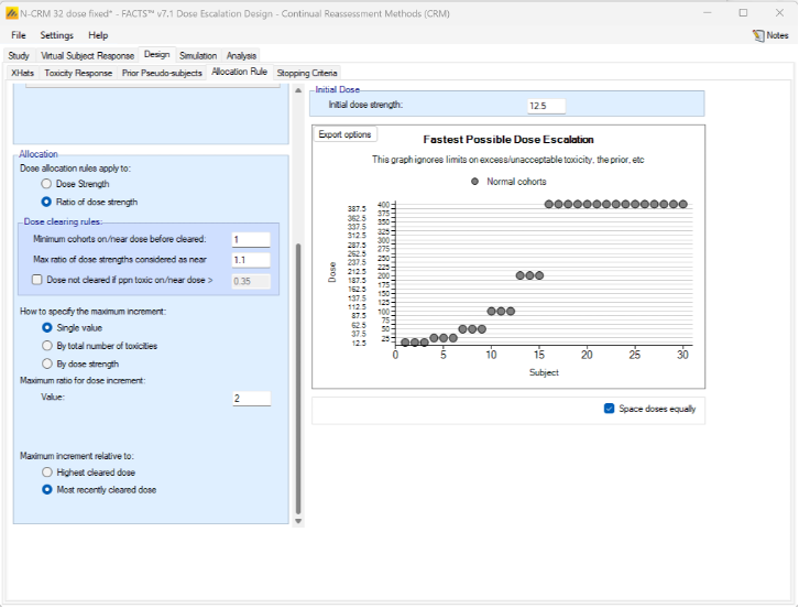
Figure 6: Doses from 12.5 to 400mg, with fixed spacing of 12.5. Showing dose escalation by dose doubling.
When requiring a certain number of cohorts to have been allocated to the estimated MTD before the trial can stop / to allow the trial to stop, we might now count cohorts on doses near the estimated MTD as counting towards that total. This is set on the Design > Stopping Criteria tab. In considering which doses are near, the same logic as on the Design > Allocation Rule tab regarding Dose Strength or Ratio of Dose Strength will be used.
- If Dose Strength is used, then on the Design > Stopping Criteria tab, we can include cohorts on nearby doses to count towards the required number of cohorts on the estimated MTD by specifying “nearby” in terms of dose strength. For example, by +/- 12.5 mg:
  
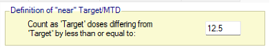
  Figure 7
- If ratio of Dose Strength is used then on the Design > Stopping Criteria tab, we can include cohorts on nearby doses to count towards the required number of cohorts on the estimated MTD by specifying “nearby” in terms of dose strength ratio. For example, by +/- 10%:
  
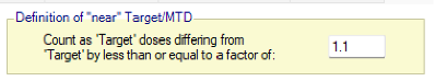
  Figure 8

Note that with Fine Grain dosing, if a band is specified for a dose to count as cleared, then the maximum cleared dose will be the maximum dose within that band, and if incrementing relative to the Maximum cleared dose, then the maximum permitted increment will be relative to the maximum dose within the cleared band.

Open Enrollment

Open enrollment (Broglio et al. 2015) can be used instead of cohort enrollment. Cohort enrolment enrolls a fixed number of subjects to a given dose, then waits until their treatment and follow up is complete (so their final status – whether they suffered a DLT (Dose Limiting Toxicity) or not – is known) before deciding on the next dose to allocate to and then recruiting the next cohort. This likely means that subjects become available for inclusion in the trial, but have to be turned away as the trial waits for the current cohort to complete. Open enrollment attempts to address this by allowing subjects to be enrolled whilst the current “cohort” is completing. However, this may come with some risk – more than a cohort’s worth of subjects may now be exposed to a new dose before we have any estimate of its DLT rate. To allow this risk to be managed, open enrollment introduces two new concepts:

When allocating to an uncleared dose, a cap can be set on the number of subjects that can be allocated to that dose who have not yet got their final results (“OE cap 1”). For example, if this number is set to 3 (to be the same as a common cohort size), after 3 subjects have been recruited and allocated to the current dose, no more subjects will be allocated to this dose until at least one of these subjects has completed. Until then, potential subjects that become available will be turned away unless backfilling is enabled (see next point below). But unlike cohort enrolment, as soon as the first of the subjects on the dose completes, a subject that comes available could now be allocated to the dose, depending on further rules explained below (frontfilling) – unless of course that subject’s result has changed the estimated MTD. Note that the trial won’t escalate beyond the current dose until the required number of subjects to clear the dose have completed. By default, the trial won’t allocate more than the number of subjects required to clear the dose until the dose is cleared, meaning if 3 subjects are required to clear a dose and 3 subjects have been allocated to this dose, even when 1 or 2 of these subjects have their final results and a new subjects is enrolled, they won’t be allocated to this dose. If this is regarded as over cautious, it can be modified by enabling frontfilling, allowing 3 subjects without final results simultaneously. In the above example, this would mean we could place a fourth subject on the dose when the result of the first subject has come in and a fifth subject as soon as the result of the second subject has come in.
When the cap on the number of subjects without final results on an uncleared dose has been reached (“OE cap 1”) new potential subjects will be turned away, unless backfilling is enabled. Enabling backfilling allows these subjects to instead be included, allocating them to a lower dose that has already been cleared. Whilst such an allocation may not contribute as much to identifying the MTD as allocating to the current dose would, it can still contribute by:
1. Increasing the information on the next lower dose can inform the estimate of toxicity on the current dose through the Bayesian logistic model.
2. Providing additional information on a dose that it may be necessary to de-escalate too if the current dose turns out to be too toxic.
It can also contribute information on other endpoints (such as efficacy). Once backfilling has been enabled, it is also possible to enable frontfilling. For more information on backfilling and frontfilling, see this section.

Assume at a given point in time we want to allocate a subject to a specific dose, denoted by “candidate dose”. FACTS allows 3 different caps to be specified on how many subjects who have not yet got their final results (i.e. are not yet complete) can be allocated to this candidate dose:

Maximum subjects without final results if dose is uncleared: As described early in this section, we encounter this cap during escalation when the candidate dose is not yet cleared. This cap takes into account subjects not yet complete on the candidate dose and any higher dose (“OE cap 1”).
Max subjects without final results if dose is cleared and below MTD: We encounter this cap when the candidate dose is cleared and below the estimated MTD (which can happen if the estimated MTD is beyond the range of available doses, when backfilling, or when allocating during the efficacy phase of a toxicity plus efficacy trial). This cap takes into account subject not yet complete on the candidate dose and any lower doses (“OE cap 2”).
Max subjects without final results if dose is cleared and at MTD: We encounter this cap when the candidate dose is cleared and the current model estimated MTD (which can happen when after clearing a dose we decide not to escalate, or after de-escalating) (“OE cap 3”).

Backfilling and Frontfilling

As described in the preceding section, Backfilling is the allocation of subjects to a lower dose when, due to restrictions, it is not possible to allocate a subject who comes available to the current dose (Dehbi, O’Quigley, and Iasonos 2021). FACTS provides a number of options to configure how backfilling behaves. Backfilling can be enabled in the Study > Study Info tab. The total sample size can be divided between the subjects allocated as part of conventional dose escalation and those allocated using backfill. When backfill is enabled, it is important to increase the total sample size and then limit the number that can be allocated using backfill, as subjects allocated using backfilling will not contribute to the escalation and the confirmation of the MTD and it’s usually important to retain sufficient sample size to achieve this aim.

When enabling backfilling, several options can be specified in the Design > Backfill Allocation tab.

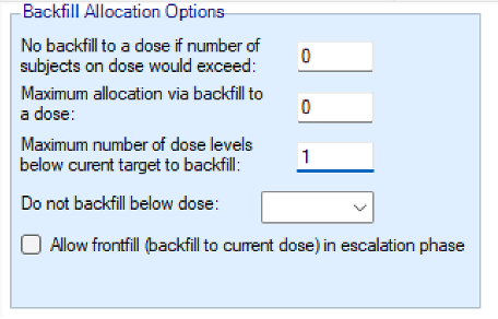
Two maximum caps can be specified on the number of subjects that are assigned in the process of backfilling to a given dose:
- an overall cap on subjects per dose that cannot be exceeded by backfill, counting also subjects that were assigned to that dose through regular allocation
- a cap on the number of subjects per dose that were allocated by backfill, counting only subjects that were assigned to that dose using backfilling.
How many dose levels below the current dose can be allocated to when backfilling. Backfilling will always be to the highest dose possible (which might be the current dose if frontfilling is enabled, otherwise it will be below the current dose). Allocation to the next highest dose might be limited either by an open enrolment cap if there are already subjects allocated to that dose who have not yet completed, or it might be limited by the backfill caps described above. If allocation to the dose below the current dose is not possible, backfilling will by default look at the dose below that (two levels below the current dose) and so on. Using this option can ensure no backfilling happens to doses that are too far below the current dose.
The lowest dose that can be allocated to when backfilling. This option is particularly useful when there is reason to believe doses below a certain level will not be effective.
Whether frontfilling is allowed – frontfilling allows allocating more subjects to uncleared doses than the number required to clear that dose (see this section).

Open Enrollment, Backfilling and Fine Grain Dosing

When using open enrolment and fine grain dosing, the interval defined on the Design > Allocation Rule tab “Delta in dose strength considered as near +/-“, or “Max ratio of dose strengths considered as near” is crucial: it is used to define the range of doses where subjects allocated to any of them count towards clearing a dose.

If dose allocation rules are selected to apply to “Dose strength”, the interval is defined “Delta in dose strength considered as near +/-“. Thus, for example, if this is set to 2, then subjects complete on doses with strength in the range 4-8 will contribute to the dose of strength 6 being cleared. At the same time, clearing the dose of strength 6 will automatically clear the dose of strength 8.
If dose allocation rules are selected to apply to “Ratio of strength”, the interval is defined “Max ratio of dose strengths considered as near“. Thus, for example if this is set to 1.5, then subjects complete on doses with strength in the range 4-9 will contribute to the dose of strength 6 being cleared. At the same time, clearing the dose of strength 6 will automatically clear the dose of strength 9. These ranges also apply when assessing “OE cap 1-3”, and how many subjects have been allocated overall, or via backfilling. In backfilling, FACTS checks each dose strength and the doses in its “near” interval range, at (if frontfilling) or below the current dose, until the first dose strength is found where backfilling can take place.

The FACTS N-CRM GUI

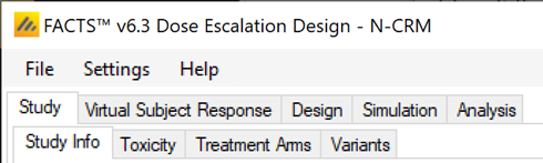
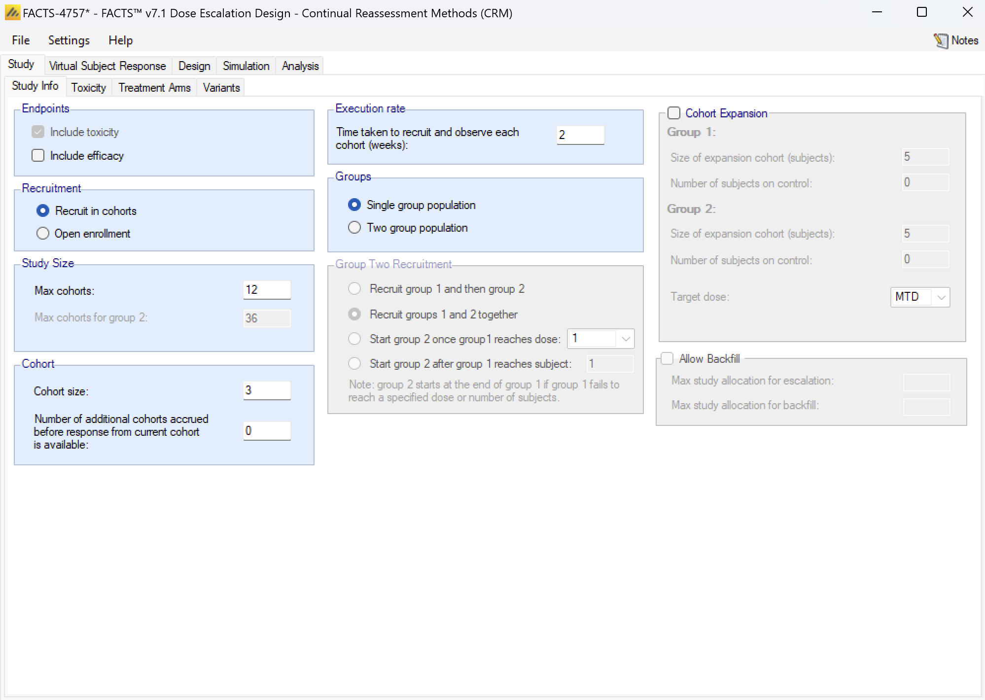
The FACTS N-CRM GUI conforms to the standard FACTS GUI layout, with information and displays divided across various standard tabs (Figure 12).

The Study Tab has sub-tabs for entering Study Information and specifying the Treatment Arms (doses) available in the study. This is where the user specifies the ‘given’ requirements, or constraints, of the trial to be designed.
The Virtual Subject Response tab has sub-tabs for specifying Explicitly Defined response scenarios to simulate and loading External data files of simulated subject responses. This is where a set of different toxicity rates per dose are specified that should represent the expected ‘space’ of the expected dose-toxicity profiles for the compound being tested.
The Design has sub-tabs for specifying the Allocation Rules, Stopping rule and Toxicity Response model. These are the design choices open to the trial biostatistician. The expected consequences of these design choices are estimated by running simulations of the trials using the various virtual subject response profiles defined.
On the Simulation Tab, the user controls and runs simulations and can view the simulation results.
On the Analysis tab, the user can use the design to analyze a specific data set and report the result of fitting the specified toxicity response model and the recommended dose for the next cohort.

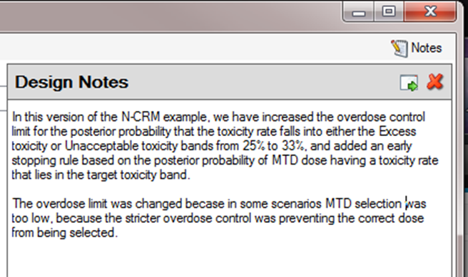
Also on the menu bar, on the right hand side of the FACTS Window, is a button labeled “Notes”; clicking this button reveals a simple “notepad” window in which the user can maintain some simple notes that will be stored within the “.facts” file (see Figure 13 and Figure 14)

The notepad window comes with two further buttons: one to change the window to a free floating one that can be moved away from the FACTCS window; and the other to close it.

The Notes field can be used for any text the user wishes to store with the file. Suggested uses are: to record the changes made in a particular version of a design and why; and to comment on the simulation results. This will help when coming back to work that has been set aside, to recall what gave rise to the different version of a design.

The Study tab

Study Info

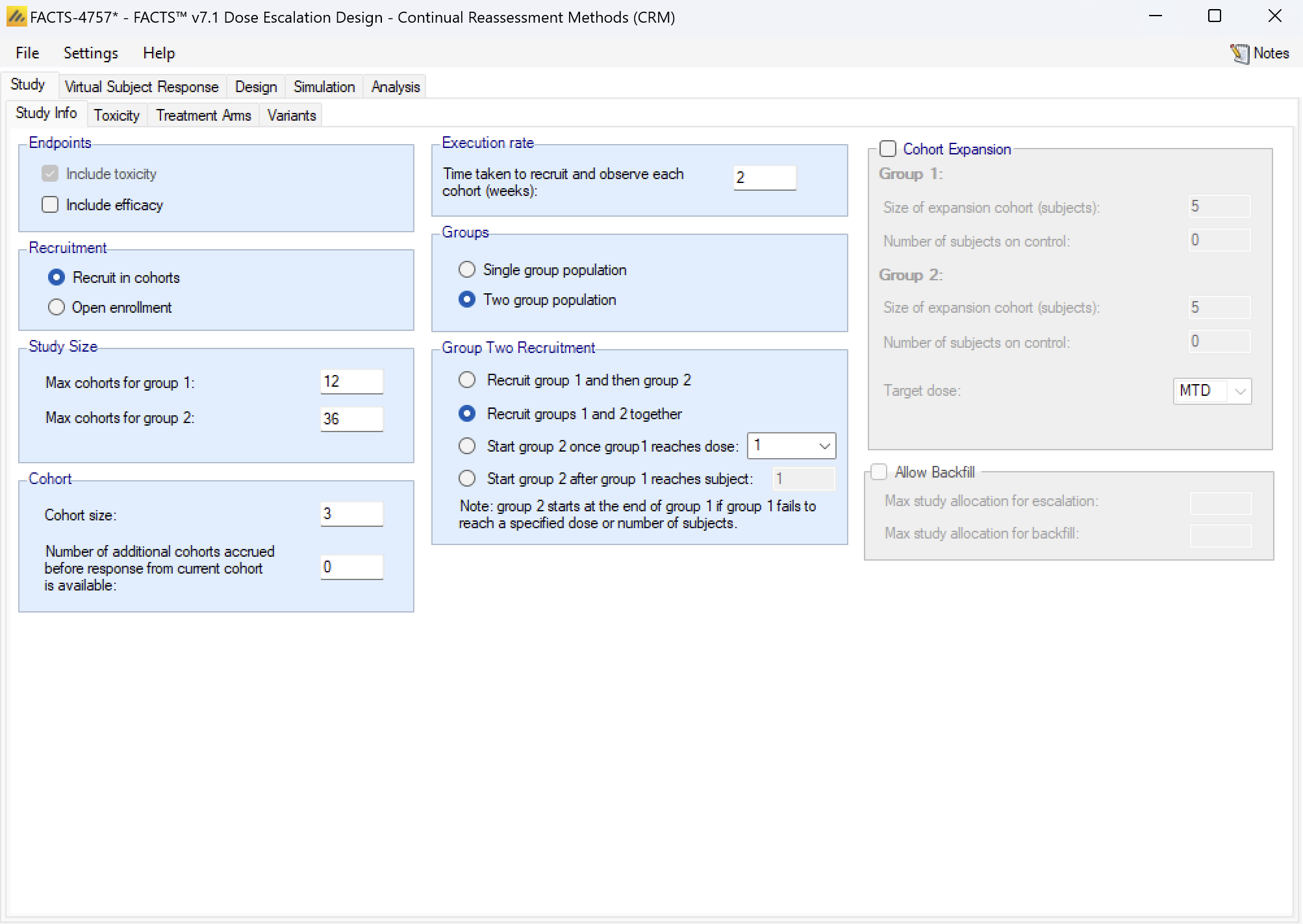
The Study Info sub-tab provides parameters for specifying:

Whether the trial has an Efficacy endpoint as well as a Toxicity one.
Whether recruitment is in Cohorts or uses Open Enrolment,
Whether the trial data is being analyzed as a single population (single group) or two groups (which could be 2 different patient types, or 2 different treatment types).
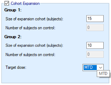
The option to specify that the trial should include an expansion cohort once the MTD has been identified.
The option (if using open enrolment) to specify the use of backfill.

Including an efficacy endpoint – this allows the trial to include a binary efficacy outcome that is observed at the same time as the toxicity endpoint. Once the MTD has been sufficiently determined further cohorts are allocated to determine the MED (Minimum Effective Dose) as long as that is below the MTD, until the maximum sample size or MED stopping rules have been reached.

Cohort versus Open enrolment: cohort enrolment is the standard way of running a phase 1 trial, a cohort of subjects of pre-determined size are treated at the current dose and the trial pauses until all the subjects in the cohort are complete, then the dose for the next cohort is determined. A phase 1 trial using Open Enrolment recruits ‘all comers’ with a cap on the number of subjects who can be treated but have not yet had a final result. Subjects that arrive whilst this cap has been reached are deemed to be ‘lost’ to the study.

If Open Enrolment and Efficacy Endpoint options are being used together, then subjects who arrive who cannot be allocated to the MTD (because the cap number of subjects awaiting a final result has been reached), can be allocated to the MED (as long as that is below the MTD).

If the trial is analyzing 2 Groups then a joint statistical model is used with options to constrain the group 2 difference in the intercept term to be +ve or -ve, and options as to whether a common or separate estimates of the slope term are used.

If an expansion cohort is included, the this is a single cohort (or one per group, if 2 groups is being used) typically much larger than used during the dose escalation, that is assigned at the end of the study to the target dose. FACTS simulates the results that arise from this cohort and a final analysis.

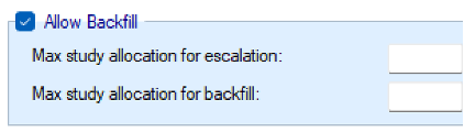
If open enrolment is being used, the further option to use backfill becomes available. The parameters on this tab for backfill, are to specify the maximum number of subjects that can be allocated for escalation, and the maximum that can be allocated in backfill. These two maximums should not total less than the overall “Max subjects” that can be enrolled. If adding backfill to a trial, usually the previous “Max subjects” becomes the “Max study allocation for escalation”, and an additional sample is allowed for backfill and added to the overall Max subjects.

If the trial has two groups the backfill maximums are the sum of the subjects in the two groups.

For Cohort enrolment, the parameters are:

Maximum Study Size, in cohorts: the maximum number of cohorts the trial can use, though designs can include conditions that cause them to stop earlier.
If the trial has two groups, the maximum number of cohorts of the second group.
Cohort size: The number of subjects in each cohort. The maximum sample size for the trial is simply: Max Trial Size (cohorts) * Cohort Size.
Cohort information delay: Normally left at zero, this allows for the trial to be simulated with cohorts recruited more quickly than if waiting for the last cohort to complete before treating the next cohort. This allows the trial to complete in shorter time, but is likely to lead to a larger incidence of toxicities. If the delay is set to 1, the second cohort will be recruited before the results for the first cohort are available, the third cohort will be recruited after the results of the first cohort are available but before the results for the second cohort are available, and so on.
Execution rate: the time taken to recruit, treat and complete the observation of each cohort (in weeks). The value of this parameter does not affect the behavior of the simulations, but it allows a nominal “duration” of each simulation to be calculated. Unlike other FACTS simulations, this duration is not simulated stochastically, it is simply the number of cohorts * this duration. Its purpose is to give a figure to compare with open enrolment designs of the same trial.

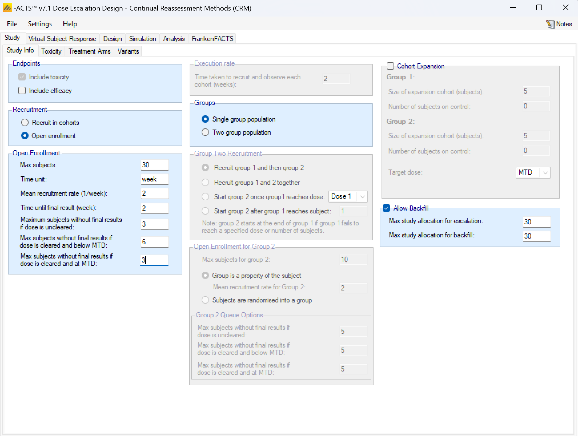
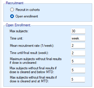
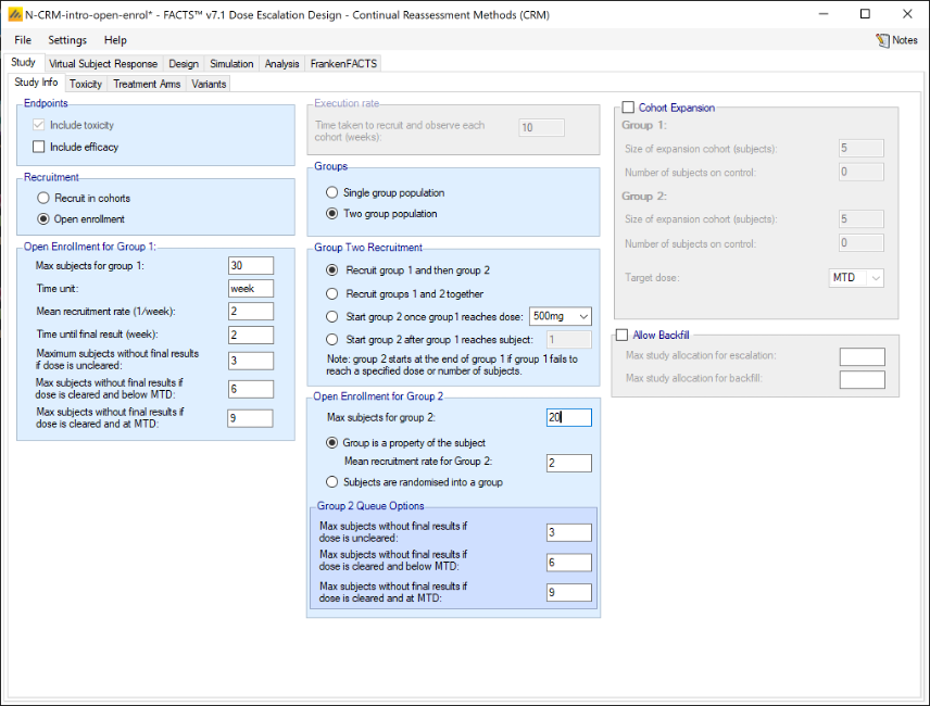
Figure 15: Study Info - Cohort Enrolment

If rather than Cohorts, subjects are recruited using open enrolment, the parameters are:

Max subjects: the maximum number of subjects who can be recruited into the study.
Time unit – this is a text string that will change the “units” label for time on graphs. This allows data to be more easily entered when the natural time unit is not “weeks”, but “days” or “months”.
Mean recruitment rate: for simulation purposes this is the average number of subjects who will be expected to be available for recruitment during each time period. Recruitment is simulated using a standard Poisson process.
Time until final result: the time for each subject for their final result to become available. This is simulated as a fixed length of time that is the same for all subjects.
Maximum subjects without a final result: the cap on the number of subjects on the current dose or a backfill dose (if backfill is enabled) who can be recruited but not yet completed. This is also known as the ‘maximum queue length’. Subjects arriving and available for recruitment while the number of subjects on this dose who have been treated but have not yet completed is at this maximum, are dropped and assumed no longer available for recruitment. Once the current subjects complete the study has to await further new subjects to become available. There are three caps:
- Maximum subjects without final results if the dose is uncleared. This allows the design to be cautious when a new dose is used for the first time.
- Maximum subjects without final results if dose is cleared and below MTD. This allows a larger number of subjects without final results to be recruited at backfill doses or at the current escalation dose if backfill to the current escalation dose (“frontfilling”) is enabled, or at the MED in the efficacy phase of a trial that includes an efficacy endpoint.
- Maximum subjects without final results if dose is cleared and at MTD. This allows us to be more cautious if the model thinks all doses are toxic or if we are allocating at the model MTD and don’t want to expose too many subjects.
Backfill – this can be enabled. Backfilling is the allocation of subjects to a dose below the current target dose, if the number of subjects allocated to the current target dose without final results has reached the maximum. Further parameters for backfill are set on the “Backfill” tab under the “Design” tab. On this tab, if backfill is enabled, two sub-maximums can optionally be specified:
- the maximum number of subjects who can be allocated as part of usual allocation for escalation and MTD determination (and MED if efficacy is included in the trial),
- and the maximum number of subjects who can be allocated as part of “backfill”.

Groups: a trial can be analyzed as a “single group” or as “two groups”. If analyzed as a single group, then all subjects are assumed to be the same and treated the same (except for the difference in the dose strength). If analyzed as two groups this allows either:

The subjects can be simulated as coming from two similar but distinct groups such as: adults and children, first line or recurrent, having some concomitant treatment or not. The separation into the two groups is based on some property of the subject.
Or the subjects can be simulated as having been allocated (possibly randomized) to one of two versions of the treatment, with the same rang of dose strengths and differing in some other way such as dosing schedule, treatment duration or combination with an additional treatment. The separation of the subjects into the two groups is under the control of the protocol.

In either case the same analysis options are available (hence we use the generic term “groups” to describe this feature).

If enrolment is by cohort, the there are two separate “maximum study sizes” in cohorts – one for each group.

The Group 2 recruitment, while it overlaps in time with the Group 1 recruitment, is simulated as being in lock-step and the recruitment of the cohort in each group is concurrent and analyzed when both are complete. In the ‘cohorts.csv’ files that are output, the cohort numbers indicates which cohorts were concurrent. The options are:

To recruit group 1 first then recruit group 2 only when group 1 is complete.
To start recruiting both groups in parallel from the outset.
To start recruiting group 2 once group 1 has reached a specified dose. The first group 2 cohort is recruited in parallel with the next group 1 cohort after the first group1 cohort has been allocated the specified dose (if cohorts can be accrued before the cohort before has completed, the group 2 is accrued too – it does not wait until the group 1 cohort completes unless the next group 1 also waits).
To start recruiting group 2 once group 1 has recruited a specified number of subjects. The first group 2 cohort is recruited in parallel with the next group 1 cohort after the specified number of subjects had been recruited into group 1.

If enrolment is open then there are options similar to the cohort enrolment to control when enrolment into group 2 starts:

To recruit group 1 first then recruit group 2 only when group 1 is complete.
To start recruiting both groups in parallel from the outset.
To start recruiting group 2 once group 1 has reached a specified dose. The first group 2 subject can be recruited after the first group1 subject has been allocated the specified dose.
To start recruiting group 2 once group 1 has recruited a specified number of subjects. The first group 2 subject can recruited after the specified number of subjects had been recruited into group 1.

But in addition the user specifies the maximum number of subjects in Group 2 and how the recruitment is to be simulated:

With the group membership a property of the subject – along with a mean recruitment rate for group 2.
With subjects randomized between the two groups (the randomization is fixed at 1:1).

The user specifies the three “Maximum subjects without final results …” for the second group.

If backfill is enabled, the backfill totals apply to the total of the subjects on both groups.

Figure 18: Study info - 2 group options with open enrolment

Enable Final Expansion Cohort: if this is enabled a final cohort of specified size will be allocated the dose selected as MTD at the end of the N-CRM phase of the study:

If the study includes a control arm, the number of subjects in this expansion cohort to be allocated to control is also specified.
If the study has two groups, two separate expansion cohorts will be allocated, their sizes are set separately.
If the study includes observing efficacy then the target dose can be changed from MTD to MED or OSD.

Simulating an additional efficacy outcome is simply specified by checking the “include efficacy” checkbox.

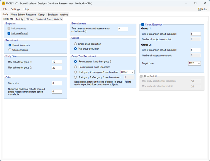
Figure 20: Study tab with “Include efficacy” checked

Simulating an efficacy endpoint can be combined with all the other features (two groups, open enrolment, backfilling) already discussed, as well as with ordinal toxicity and fine grain dosing that are described below.

Currently there are two significant limitations to the simulation of an efficacy endpoint:

The endpoint is assumed to be dichotomous.
The endpoint is assumed to be observable at the same time as toxicity.

We hope to lift these restrictions in a later version of FACTS.

Toxicity

The Toxicity sub-tab provides parameters for specifying:

Whether toxicity should be simulated as dichotomous or ordinal. If simulated as Ordinal, toxicity can be simulated as a 1-3 scale or 1-4 scale. In both cases ‘1’ is “no-toxicity”, 2 is “mild toxicity” and 3 is the toxicity of interest (from the point of view of defining the MTD, target toxicity band and Overdose Control. If a four category scale is selected, 4 is “sever toxicity” or death. Choosing whether to model the ordinal response is a separate option and is present on the Design > Toxicity Response tab.
Type of target: this allows the user to specify whether the dose selection targets “the dose who’s estimated toxicity rate is closest to a specified target rate” or “the dose with the highest posterior probability of having a toxicity rate in a target band”. The former is the target rule used in the original CRM papers ((O’Quigley, Shen, and Gamst 1999), (deMoor et al. 1996), and the latter rule was introduced in (Neuenschwander, Branson, and Gsponer 2008).
Toxicity target (only displayed if the type of target is “a single dose”): this allows the target toxicity rate to be specified and whether the target dose is the one nearest, the one nearest but with a lower rate or the one nearest but with a higher rate.
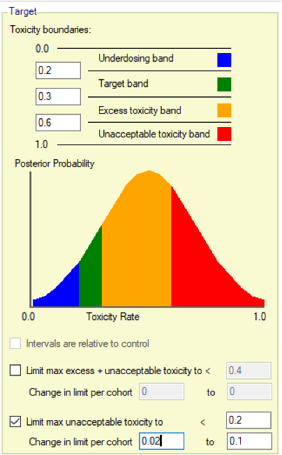
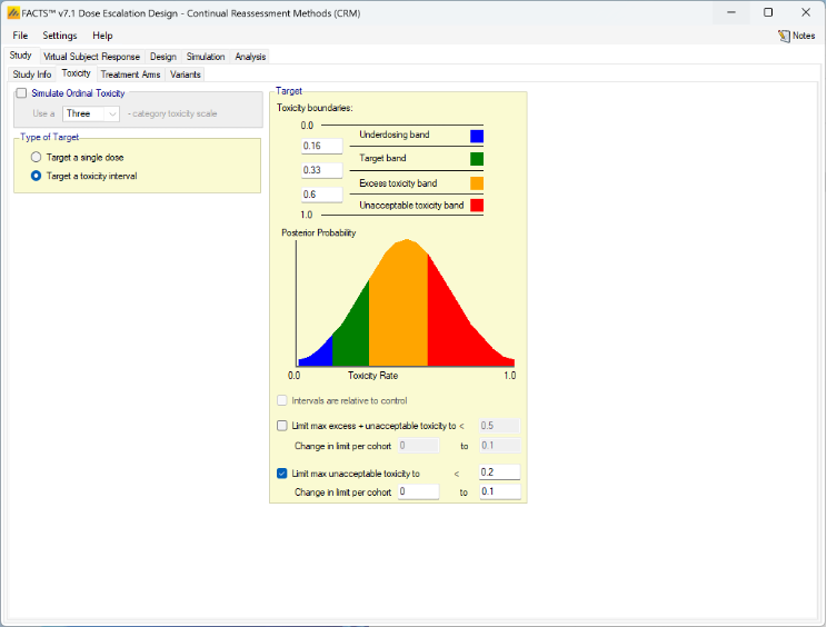
Target: this panel allows the target toxicity bands to be specified along with overdose control limits. The panel is displayed and enabled even if the target type is “a single dose” to allow overdose control limits to be specified.
Type of Target: controls the selection of the dose for the next cohort – this can be to target a single dose (to replicate the original CRM behavior, see this section) or to target the dose with the highest probability that its toxicity rate lies in a target band.

Figure 21: Toxicity tab targeting a toxicity band

Targeting a Toxicity Interval

Targeting a toxicity band or interval is an innovation introduced with the N-CRM design, unlike other CRM designs that select the dose that is expected to have a toxicity response closest to the desired tolerated limit, the N-CRM selects the dose that has the highest posterior probability of having a toxicity rate in a target toxicity band. This has the advantage of a) having a clearer probability statement and b) having in addition probability statements about the probability of under and overdosing (the toxicity rate being below or above the target toxicity band).

The uncertainty in the estimate of toxicity at each dose is expressed by calculating the posterior distribution of the estimate of the rate of toxicity at each dose and calculating the proportion of that distribution that falls in to each of 4 bands of toxicity: ‘Under-dosing’ (toxicity so low that it is likely that a higher dose could be used), ‘Target’ toxicity (we want to select doses whose toxicity rate is most likely to be in this band), ‘Excess’ toxicity (toxicity higher than desired) and ‘Unacceptable’ toxicity.
- Under-dosing: this band always starts at 0.0; the user specifies the upper bound.
- Target band: this band always starts at the upper-bound of the under-dosing band; the user specifies the upper bound.
- Excess toxicity: this band always starts at the upper-bound of the target band; the user specifies the upper bound.
- Unacceptable toxicity: this band always starts at the upper-bound of the target band, with an upper bound of 1.0. The graph shows the width of the different bands using a simple, fixed, example posterior probability distribution of a toxicity rate.
Intervals are relative to control: if a control arm is included in the study, then toxicity bands can be defined as the difference in toxicity rate relative to control. Negative differences (a lower toxicity rate than control) are always treated as under-dosing. To enable this option it is necessary to first go to the Study > Treatment Arms tab and select Include Control.
Limit max excess/unacceptable toxicity: the ‘overdose control’ in terms of a maximum allowed posterior probability that a dose’s toxicity rate lies in either the ‘Excess’ or the ‘Unacceptable’ toxicity bands. Any dose with a posterior probability of having a toxicity rate in either of these two bands that is higher than the specified limit, cannot be selected for allocation to the next cohort, nor selected as MTD at the end of the study (this gives rise to slightly different results compared to those in (Neuenschwander, Branson, and Gsponer 2008) where the overdose control was not applied to final selection).
It is possible to have the overdose control limit vary with the number of cohorts allocated. In particular this can be used to reduce the overdose limit as the number of cohorts (and the amount of information) grows. For example for a particular prior and final level of overdose control, it may be that initial escalation is excessively constrained, one way to allow early escalation in this setting is to use these parameters to allow an higher initial overdose control limit and gradually reduce it over time to the final desired limit. Tuning the parameters will require some iteration and simulation. A varying limit is specified by the specifying amount to change the limit by per cohort and the final limit. The amount to change by is always entered as a number in the range (0,1), whether this is an increment or decrement depends on whether the target limit is greater or less than the initial limit. Leaving the change in limit at its default of 0 means the limit does not vary.
Limit max unacceptable toxicity: as for the previous parameter, but here the overdose control is only in terms of the posterior probability that a dose’s toxicity rate lies in the ‘Unacceptable’ toxicity band.
As or the limit on excess/unacceptable toxicity it is possible to have the overdose control limit vary with the number of cohorts, see the description above.

Targeting a single dose

It is possible to use the N-CRM design engine with a conventional CRM allocation strategy - to “allocate to the nearest / highest dose below the maximum tolerated toxicity”; this allows conventional CRM design to be simulated with some of the additional features of N-CRM:

Overdose control
Estimate both parameters of the 2 parameter logistic
The “Recommender” to analyze a specific data set.

The target is calculated by:

In the MCMC sampling loop finding the dose that meets the target criteria, a doses probability of being the target is then the proportion of times that dose meets the target criteria across the MCMC sampling.
Rather than selecting the dose with the highest probability, the dose at the 50% quantile is used. The cumulative probability of being the target is calculated over the doses in ascending dose strength, and the dose when the cumulative probability passes 50% is selected. This addresses some problems that can arise when very little data is available: that the dose with the highest probability is at one end of the dose range, but that probability is not that high, or that doses are not evenly spaced and a dose close to both its immediate neighbors may never have greater probability than both of them.

Setting the Type of Target option to Target a single dose, modifies the tab thus:

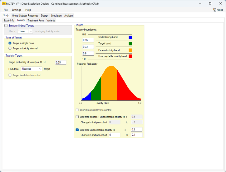
Figure 22: N-CRM, targeting a single dose, not a toxicity band

When targeting a single dose FACTS allows the user to specify:

The target toxicity rate
Whether to allocate to the dose with the mean estimate of its toxicity rate nearest the target, highest dose with a mean estimate of its toxicity rate below the target or lowest dose with a mean estimate of its toxicity rate above the target.
An option to use the toxicity rate relative to control, rather than the default of the absolute toxicity rate. To enable this option it is necessary to first go to the Study > Treatment Arms tab and select Include Control.

The definition of the boundaries of the toxicity bands is still included in order to allow the specification of overdose control limits. These are calculated and applied in exactly the same way as when targeting a toxicity interval.

Efficacy

If include efficacy has been checked on the Study Info tab, a simple additional input page is included:

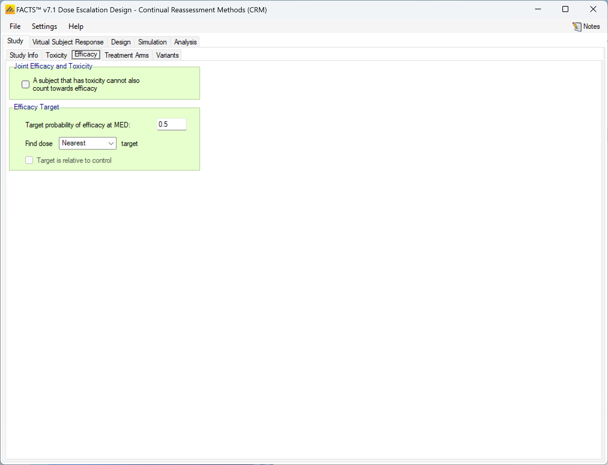
If simulating and modelling an efficacy endpoint is included there are two items to be specified on this tab:

Whether a subject experiencing a toxicity can also count towards efficacy or not. If unchecked patients outcomes are simply sampled separately and a patient can both have a toxicity and an efficacy response. If checked, a patient’s toxicity outcome is sampled first, and only if there is no toxicity is an efficacy outcome sampled.
The efficacy target – this consists of:
- The target efficacy rate required for the Minimum Efficacy Dose (MED).
- Whether the target dose is the nearest dose to the MED rate, the lowest dose above the MED rate or the highest dose below the MED rate.
- If a control arm has been included, whether the target rate is absolute or relative to the observed rate on the control arm.

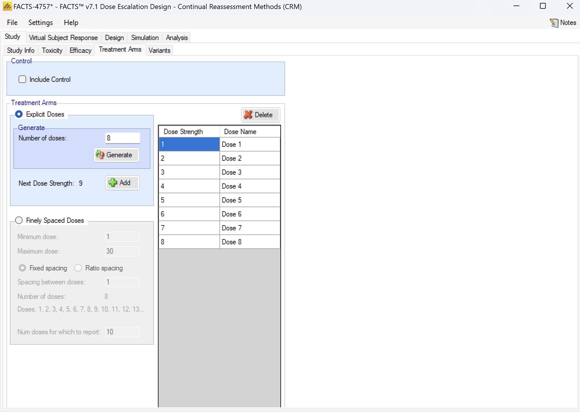
Treatment Arms

On this tab the number of treatment arms (doses) available to the study is specified. The user can either define a set of specific doses that can be used or a continuous dose range with some granularity.

Selecting Explicit Doses allows the user to specify the specific doses that can be used on the trial:

A single new dose or multiple doses can be added either by clicking “Add” or “Generate”. Initially each dose is defined by a simple integer name and level. The dose levels and dose names can then be edited on by clicking on them and entering the desired value. The dose level can also be set later on in the Design > Toxicity Response tab.
There is also the option to include a control arm. Including a control arm allows the toxicity rate to be relative to the control arm.

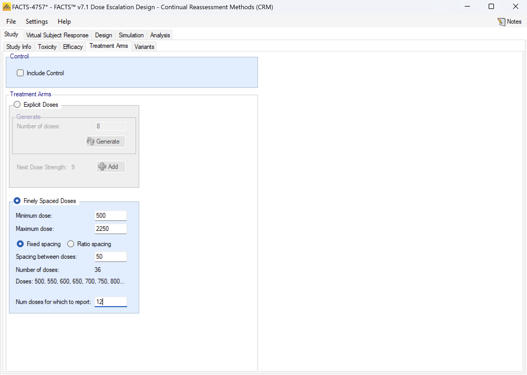
Figure 24: The Treatment Arms tab specifying explicit doses

Finely Spaced Doses

Selecting Finely Spaced Doses allows the user to specify the dose range that can be used on the trial:

The minimum and maximum dose strength to be used
The ‘granularity’ of the actual dose used, either as a fixed delta (Fixed spacing) or a dose ratio (the ratio specified must be greater than 1) (Ratio spacing).
The number of ‘bins’ or ‘doses for which to report’ – this is because FACTS will still produce summary statistics in columns, many with a “column per dose” – it is possible to use more doses than it is practical to report on (and a limit in MS Windows of 32K pixels for the width of a table means that the GUI can only display simulation results for a maximum of ~40 doses). However this limitation is only for reporting summary statistics; the dose strengths modeled and allocated in the simulations are unaffected.

Selecting ‘Finely Spaced Doses’ will also affect how some of the other parameters are specified in the FACTS GUI.

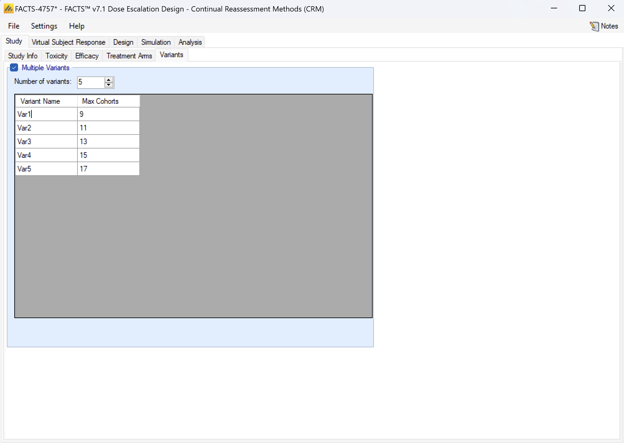
Figure 25: The Treatment Arms tab, specifying a finely spaced dose range

Variants

On this tab the user can specify that a number of design variants should be created. Currently the only design feature that can be changed is the sample size (maximum number of cohorts).

If “multiple variants” is checked then the user can specify that simulations setups should be created for each simulation scenario with versions of the design with different maximum numbers of cohorts.

The user enters the number of variants they wish to create. Then in the resulting table, enter different “Max Cohorts” for each variant.

These will then appear on the simulations tab.

If open enrolment is being used, then the enrolment cap is specified by the number of subjects.

If there are two groups then separate caps are specified for each group.

Figure 26: The Variants tab, specifying 5 variants

Virtual Subject Response

The Virtual Subject Response tab allows the user to explicitly define virtual subject response profiles. When simulations are executed, they will be executed for each specified profile.

Profiles can be specified in 3 different ways:

Explicitly: by specifying the toxicity rate to simulate at each dose. This option is only available if the available dose strengths have been specified explicitly, it is not available if a finely spaced dose range defined.
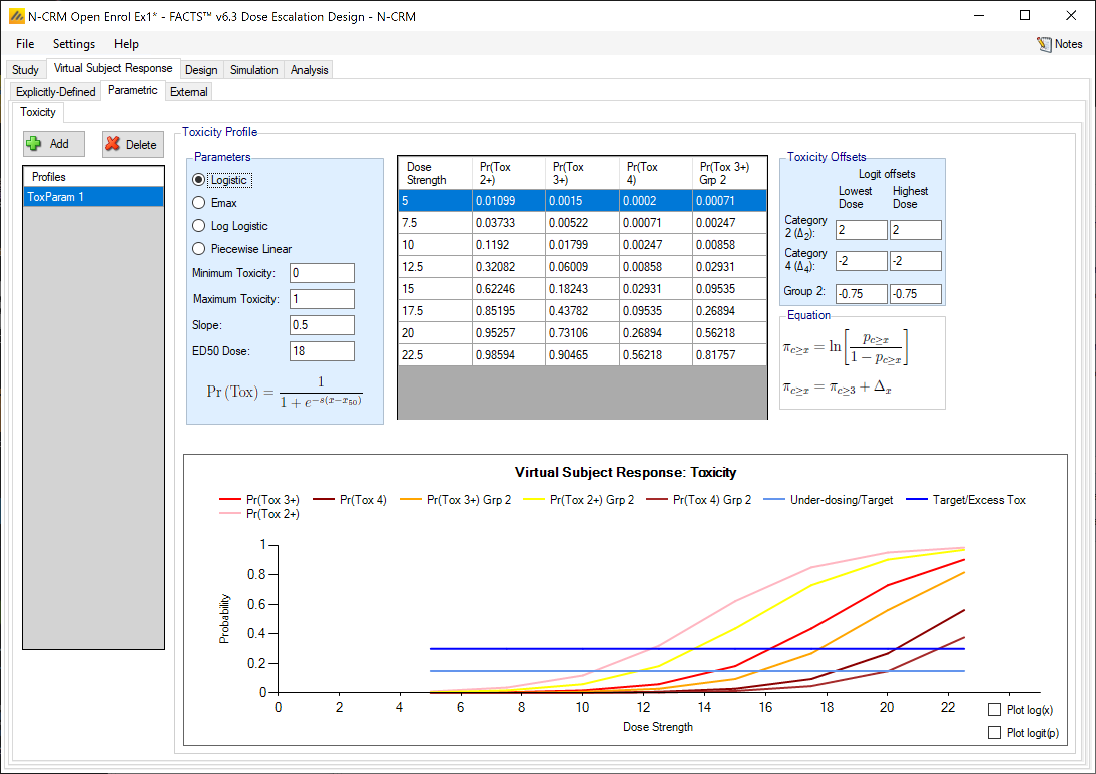
Parametrically: by selecting one of the four models and specifying the parameter values for the model, allowing the toxicity rate to simulate at each dose to be calculated.
Externally: by specifying a file of simulated subject responses at each dose strength, which will be sampled from with replacement when simulating subject responses. As in N-CRM there is a simple, single binary toxicity response per subject and there is no response profile that cannot be specified by the other methods. The mechanism is provided here more for consistency with the other FACTS interfaces.

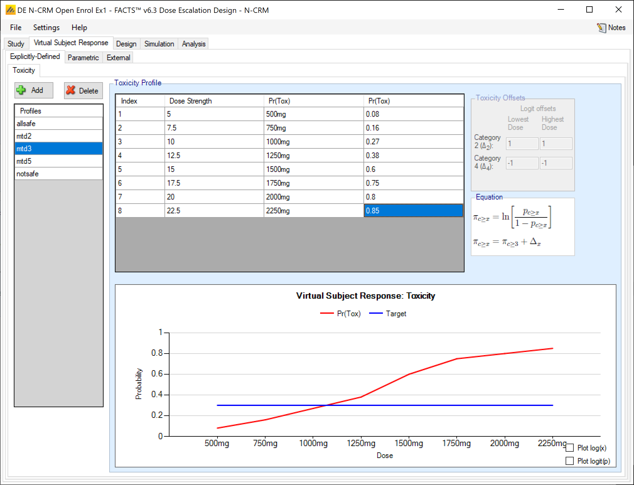
Explicitly Defined

Toxicity profiles may be added, deleted, and renamed using the table and corresponding buttons on the left hand side of the screen in Figure 28. The user enters the toxicity rate to simulate at each dose into the Probability of Toxicity column of the table, and the graphical representation of these toxicity values updates accordingly.

This form of toxicity profile is not available if the dose range is “finely spaced” – typically this means there are too many doses for it to be practicable to enter toxicity rates for all of them. When using “finely spaced” doses the toxicity rates to be simulated have to be specified using parametric models (see the next section).

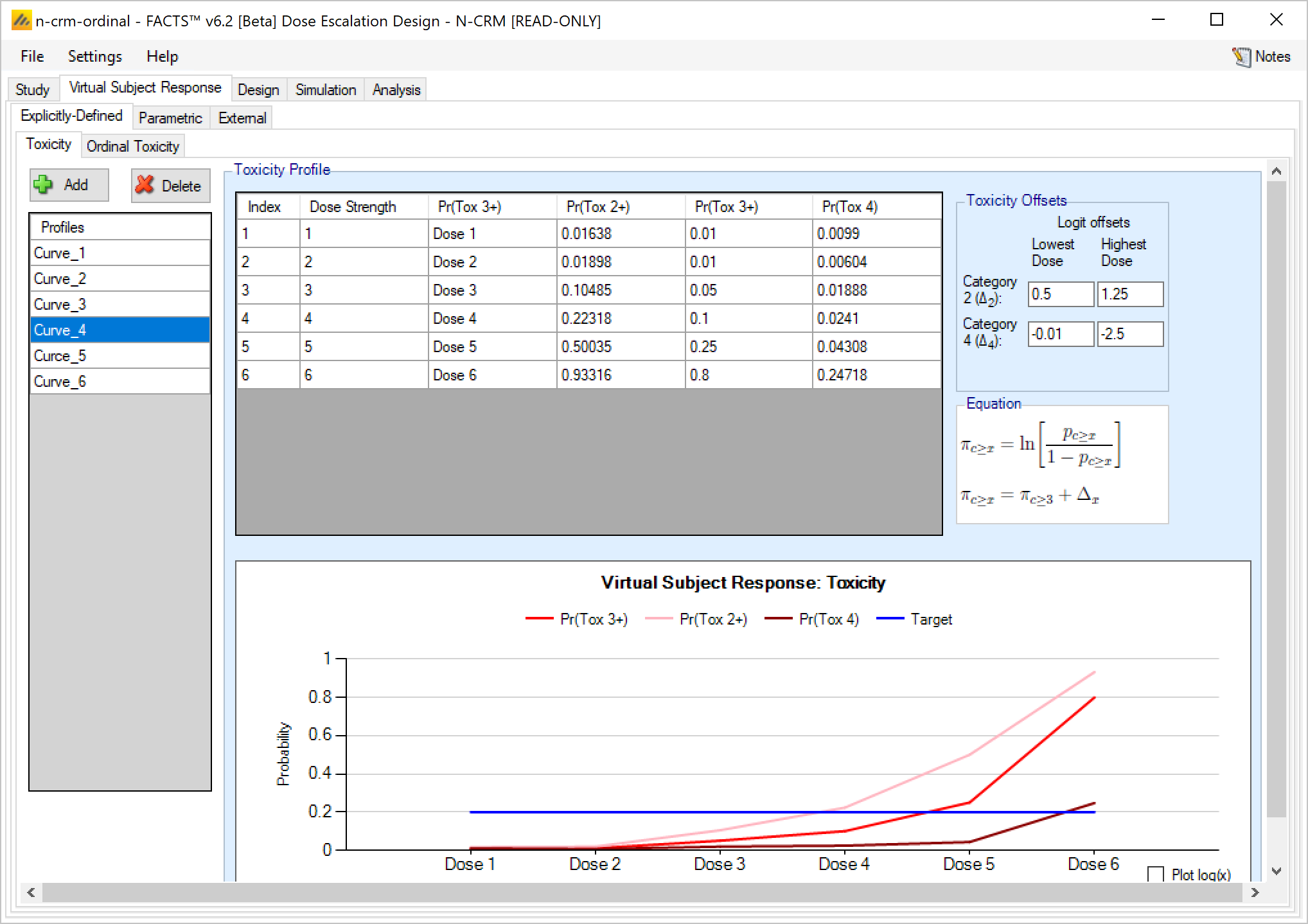
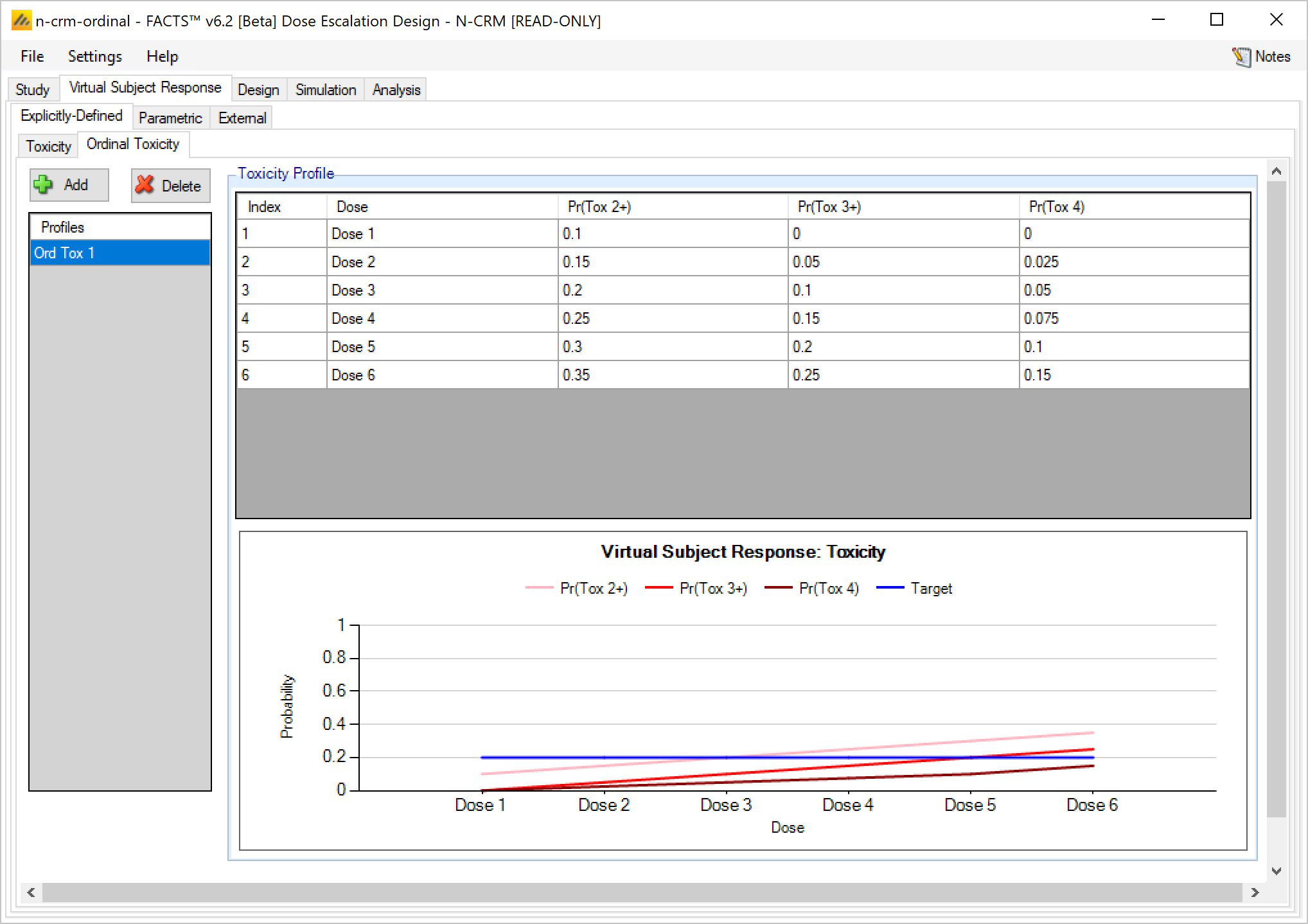
Figure 27: Explicitly defined toxicity - binary endpoint

If the design is using ordinal toxicity, the toxicity response rates can be specified either:

On the “Toxicity” tab by specifying the category 3 or greater toxicity rate at each dose and then two offsets – one for the category 2 or greater rate and one for the category 4 rate.
On the “Ordinal Toxicity” tab by separately specifying the toxicity rates for each category of toxicity at each dose.

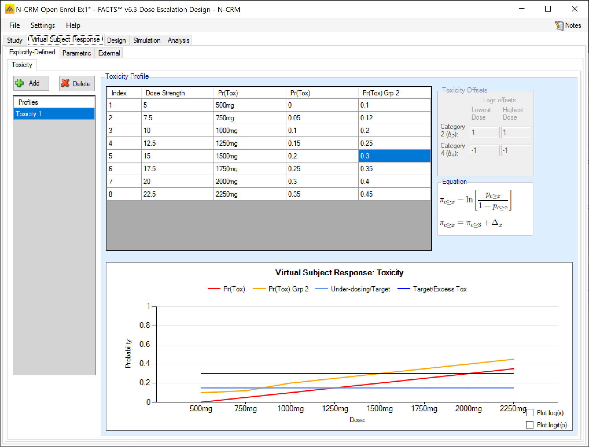
Specifying offsets: to ensure that the specified category 3 rate plus the category 2 offset doesn’t sum to more than 1, or the category 3 rate plus the -ve category 4 offset sum to less than 0, the offsets are applied to the logit of the category 3 toxicity rate.

Thus for the category 2+ rate:

\[ ln(\frac{p_{2+}}{1-p_{2+}}) = ln(\frac{p_{3}}{1-p_{3}} + \Delta_2) \]

where:

\(p_{2+}\) is the probability of observing a category 2 or greater toxicity at a dose
\(p_3\) is the probability of observing a category 3 or greater toxicity at a dose
\(\Delta_2\) is the difference in the log odds between the two probabilities

The offset is defined at the lowest dose and highest dose and then varied linearly with dose strength at the intermediate doses. The plot of the curve can either use Pr(Tox) or Log-odds(Tox) as the y-axis and dose strength or log(dose strength) as the x-axis. A graph is displayed of the toxicity rates that have been entered, and the category 2+ and category 4 toxicity rates if applicable. This graph, as with all graphs in the application, may be copied to the clipboard or to a file using the “right-click” menu.

Figure 28: Virtual Subject Response – Explicitly-Defined – ordinal endpoint

Explicitly defined – Ordinal Toxicity

If simulating ordinal toxicity an alternative option is to explicitly specify the rate at each toxicity level at each dose. This can be done under the Virtual Subject Response > Explicitly Defined > Ordinal Toxicity tab.

Explicitly defined toxicity – when simulating 2 groups

If simulating toxicity as a binary outcome, when simulating 2 groups, the tab displays two Pr(Tox) columns, one for each group, and the user enters the toxicity rate to be simulated at each dose for each group.

Figure 30: Explicitly defined toxicity - 2 groups

If simulating 2 groups and ordinal toxicity, then on the explicitly defined tab once again the tab displays two Pr(Tox) columns, one for each group, and the user enters the toxicity rate to be simulated at each dose for each group. As for a single group the Category 2 toxicity and Category 4 (if using) toxicity rates are defined by defining log odds offsets at the lowest and highest dose. Specification is limited to a single set of offsets that are applied to both groups.

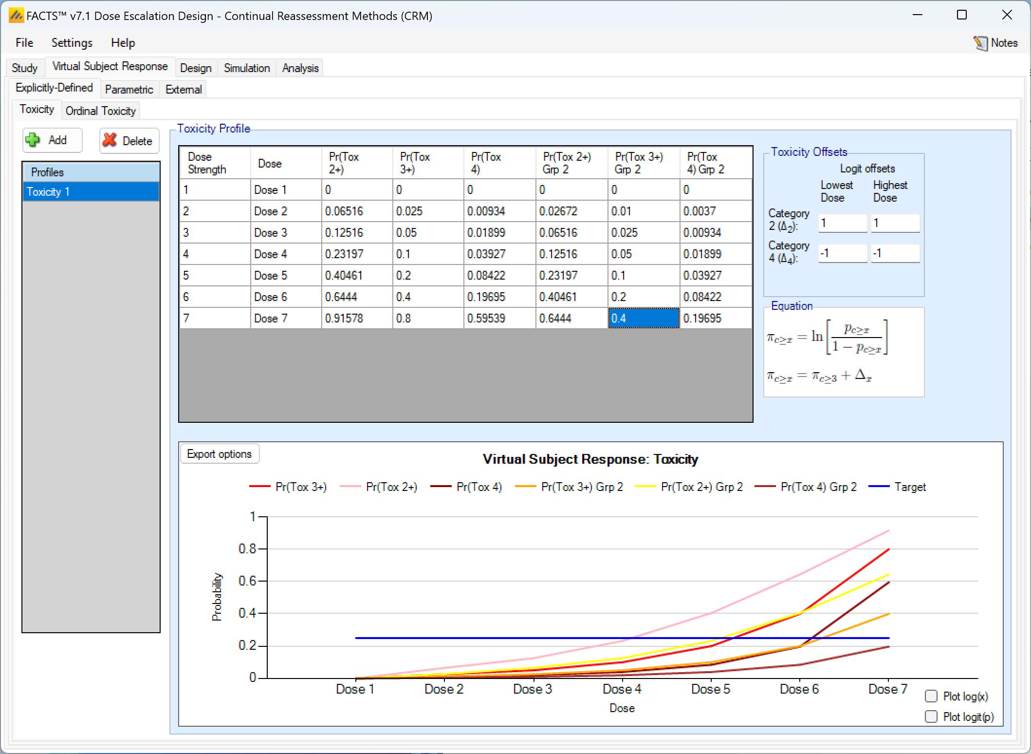
Figure 31: Explicitly defined toxicity - 2 groups and ordinal offsets

As in the single group case in addition to the Category 3 toxicity rates that are editable, columns showing the Pr(Tox 2+) and Pr(Tox 4) are shown, but these are not editable and derived from the Pr(Tox) rates and the offsets that have been specified. The ordinal toxicity rates are only shown for group 1.

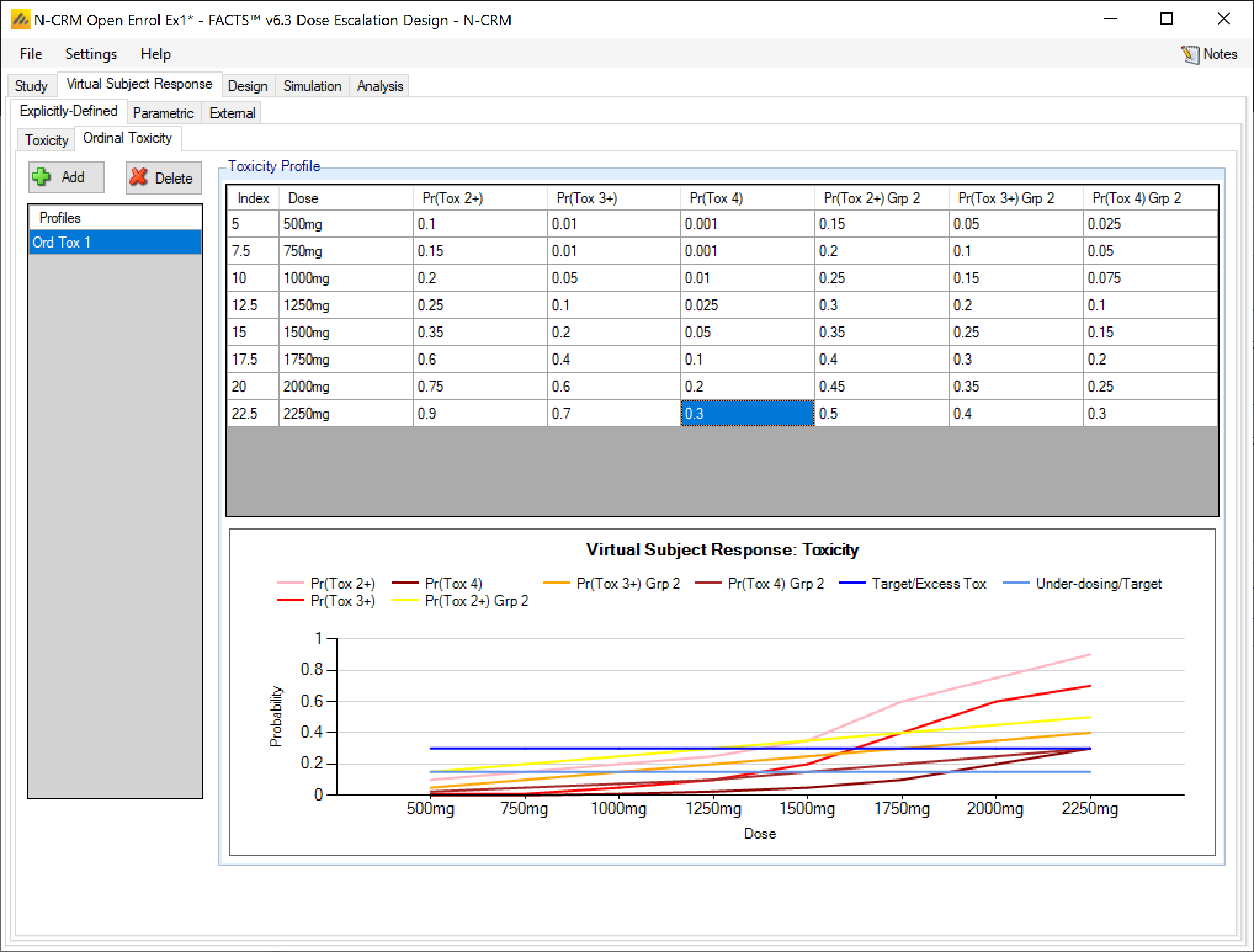
Explicitly defined – Ordinal Toxicity with 2 groups

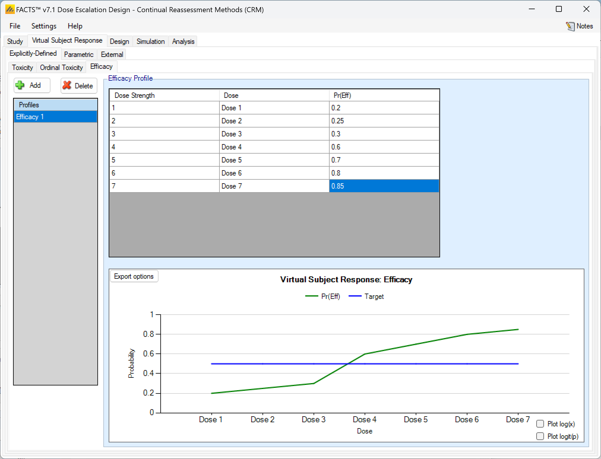
Efficacy response profiles

Entering efficacy response profiles is very similar to entering toxicity profiles. FACTS will construct scenarios to simulate of every combination of toxicity and efficacy response profiles.

Explicitly Defined – Efficacy

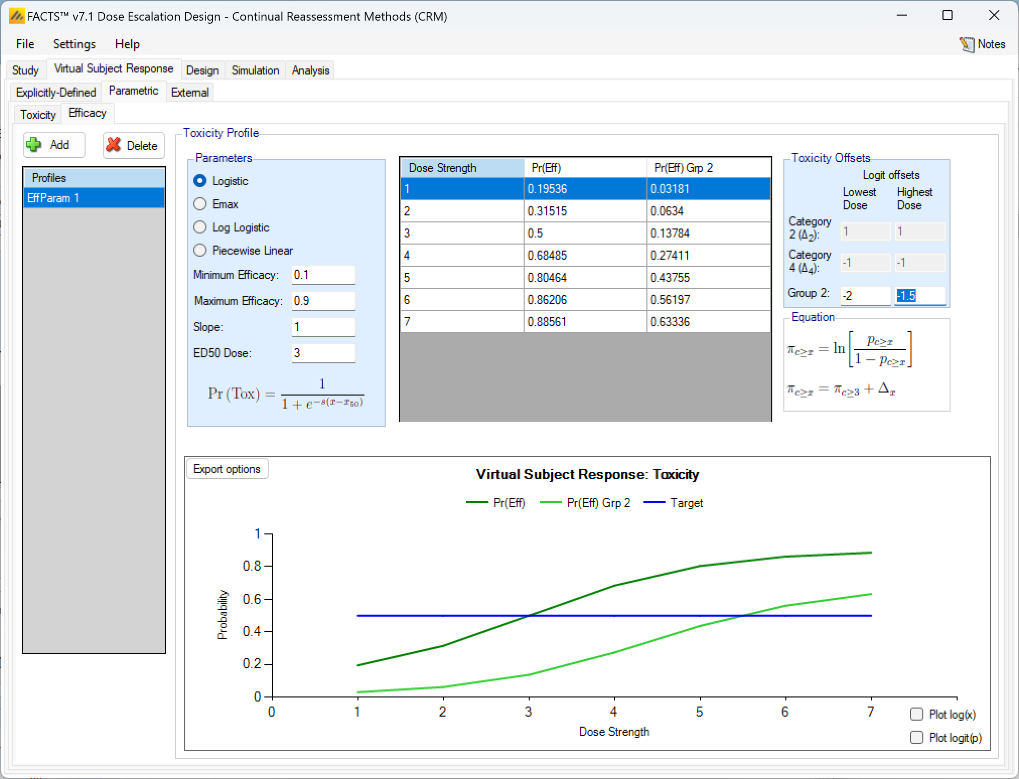
Efficacy profiles may be added, deleted, and renamed just like toxicity profiles. The user enters the efficacy rate to simulate at each dose into the Probability of Efficacy column of the table, and the graphical representation of these efficacy values updates accordingly.

As with toxicity this form of efficacy profile is not available if the dose range is “finely spaced” – typically this means there are too many doses for it to be practicable to enter efficacy rates for all of them. When using “finely spaced” doses the efficacy rates to be simulated have to be specified using parametric models (see the next section).

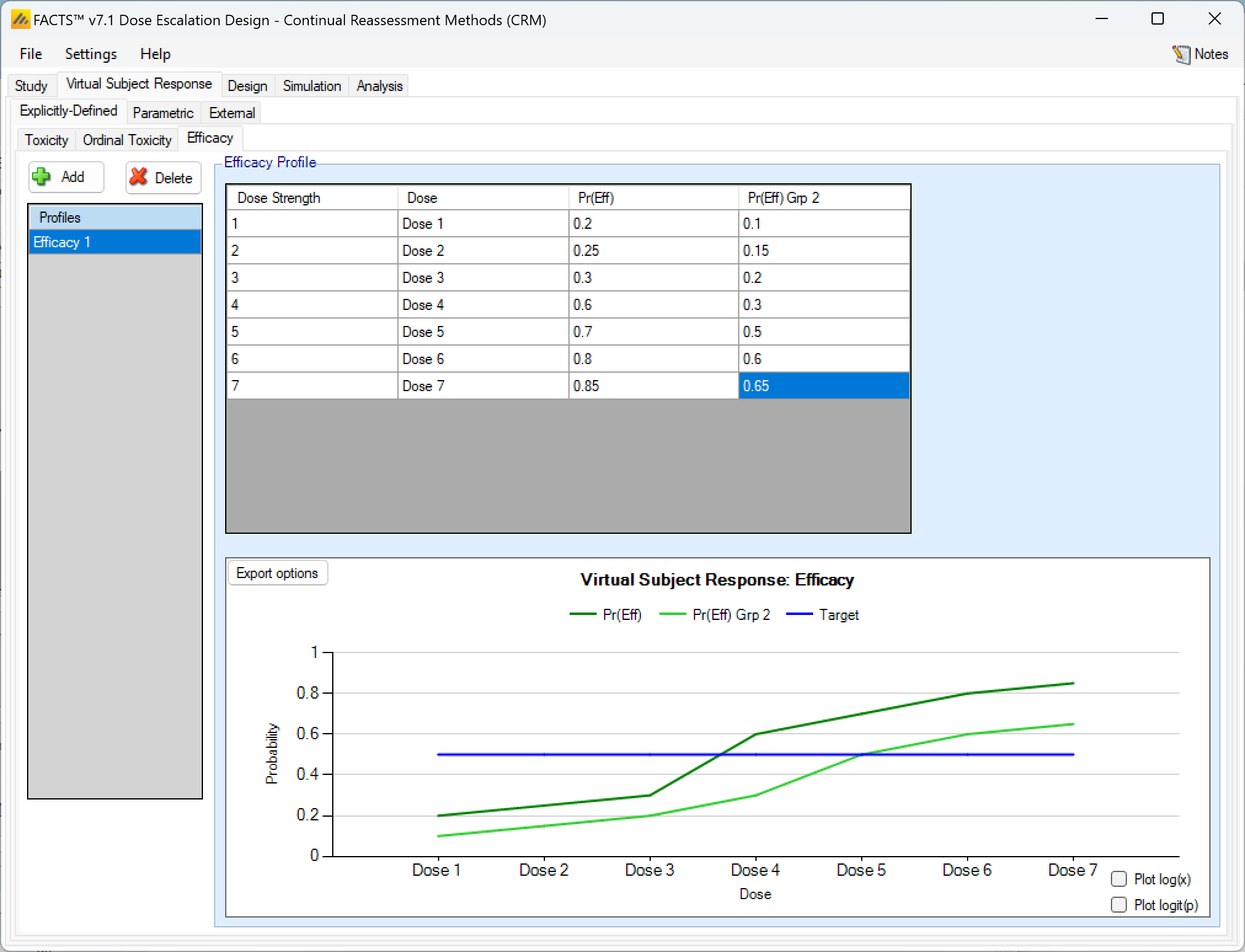
Figure 33: Efficacy virtual subject response, explicitly defined

Explicitly Defined – Efficacy with two groups

If the design included 2 groups, when explicitly defining an efficacy response profile, there is simply a second column of efficacy response rates to enter:

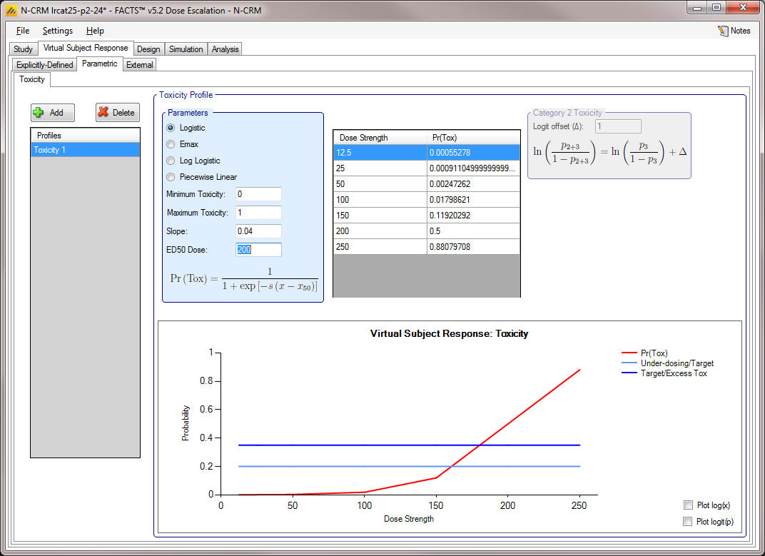
Figure 34: Explicity defined efficacy response profile with 2 groups

Parametric

Toxicity scenarios may be added, deleted, and renamed using the table and corresponding buttons on the left hand side of the screen. The user selects the model to use to determine the toxicity rate to simulate at each dose, and specifies the values of the model’s parameters. The graphical representation of these toxicity values updates accordingly.

The graph may be copied using the context menu functionality described in the previous section.

Four models are available:

Logistic: the probability of toxicity at dose x is given by: \(P_x=\frac{1}{1+e^{-s(x-x_{50})}}\) with user specified parameters, \(s\) (slope) and \(x_{50}\) (the ED50 dose). Note this can be fitted exactly by the two parameter logistic with linear effective doses \(\hat{x}=x-x_{ref}\) when \(\beta=s\) and \(\alpha=\beta*(x_{ref}-x_{50})\)
Emax: the probability of toxicity at dose \(x\) is given by: \(P_x=\frac{x}{x+x_{50}}\) with user specified parameter \(x_{50}\).
Log Logistic: the probability of toxicity at dose \(x\) is given by: \(P_x=\frac{1}{1+e^{-s(ln(x)-ln(x_{50}))}}\) with user specified parameters, \(s\) (slope) and \(x_{50}\) (the ED50 dose). Note this can be fitted exactly by the two parameter logistic with log effective doses \(\hat{x}=ln(\frac{x}{x_{ref}})\) when \(\beta=s\) and \(\alpha=\beta*ln(\frac{x_{ref}}{x_{50}})\)
Piecewise linear: with the probability of toxicity specified at a series of knots, with the probability linearly interpolated between knots.

Figure 35: Virtual Subject Response - Parametric Toxicity tab

If Ordinal toxicity is being simulated then the category 2 and greater toxicity rates and category 4 toxicity rates are specified using the logit offset methods as on the Explicitly-Defined > Toxicity tab.

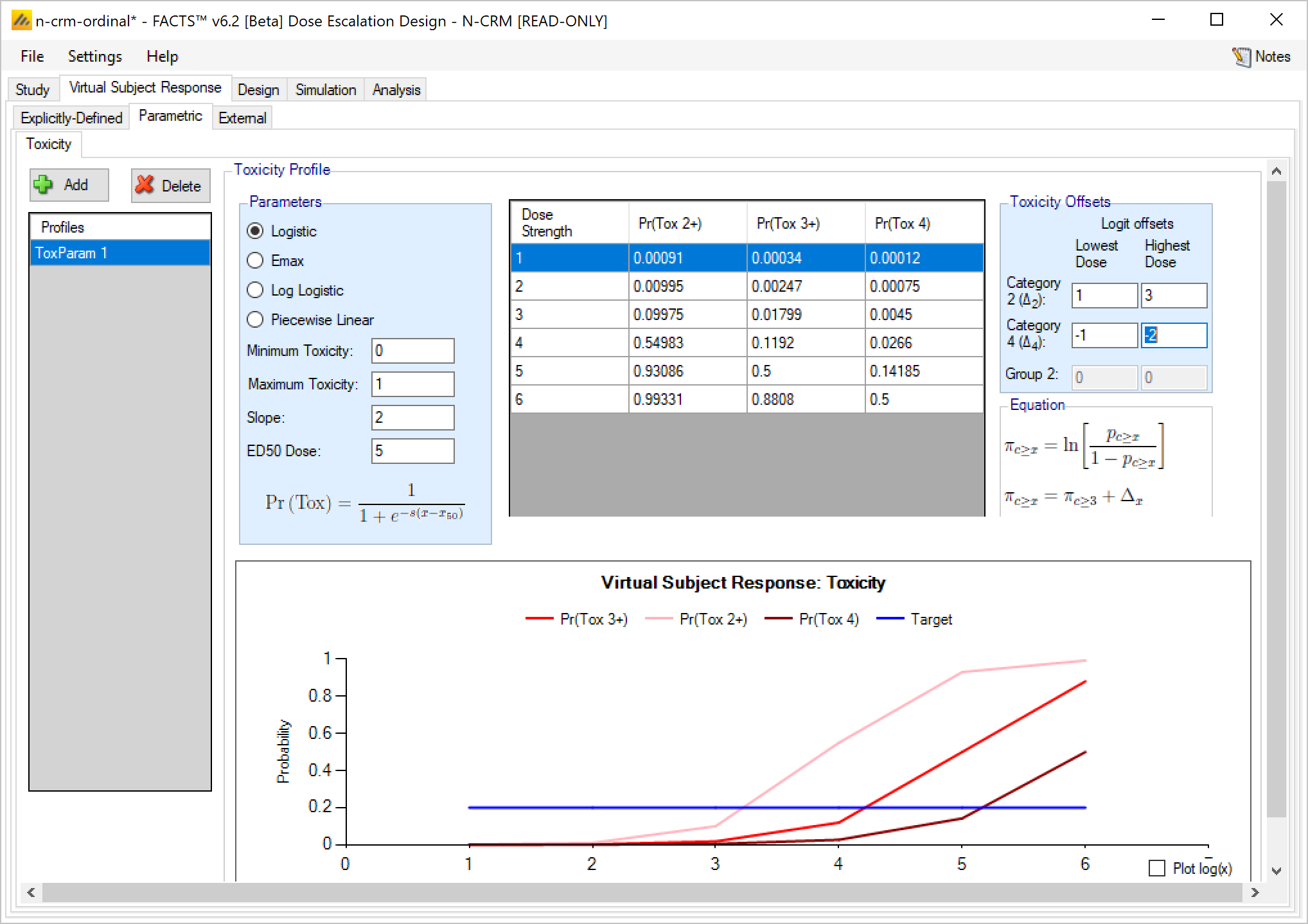
Figure 36: Virtual Subject Response - Parametric Toxicity tab with Ordinal toxicity

If Ordinal Toxicity and 2 groups are being simulated then both the Cat 2+ and Cat 4 toxicities and the Group 2 toxicities are defined using the logit offset methods.

Figure 37: Parametric definition of ordinal toxicity response with 2 groups

Parametric efficacy response

Parametric efficacy response profiles function exactly like toxicity profiles, with the same parametric models to choose from and if 2 groups are present the response of the second group is again defined by 2 log-odds offsets, one at the lowest dose and one at the highest.

External

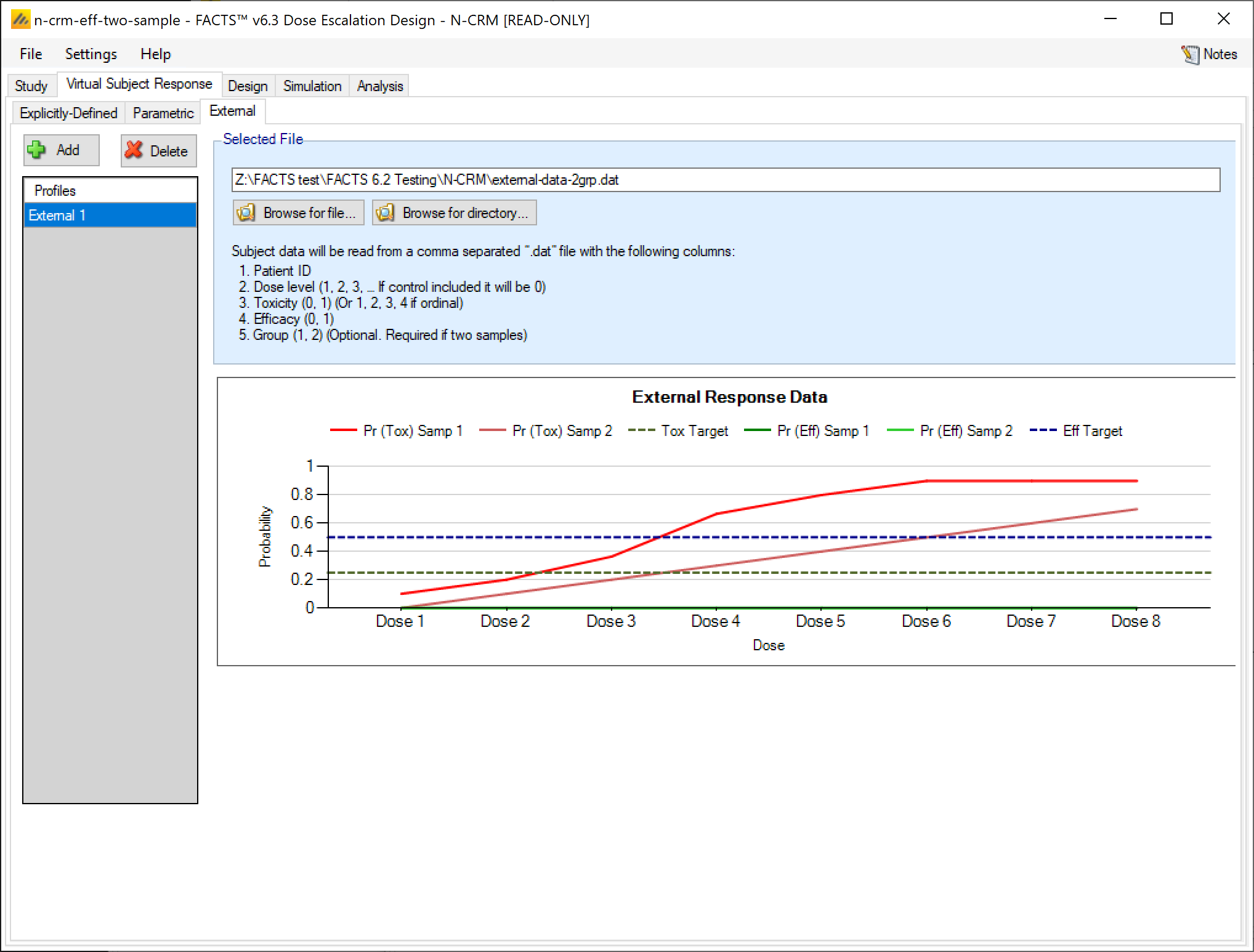
Subject response data may be simulated from a PK-PD model in place of, or in addition to, choosing a response model from FACTS. The importing of subject response data (which must be in the form specified in the System Requirements Document) may be done from the External Files sub-tab depicted below (Figure 39).

The supplied data should be in the following format: an ascii file with data in comma separated value format with the following columns:

Patient id
Dose index (1, 2, 3,… if a Control is to be included it should be index 0) this is not the user settable dose name or dose level
Toxicity (0,1)
Efficacy (0. 1) even if efficacy not being simulated this value must be present
Group (*1, 2) only required if groups are being simulated

The GUI requires that the file name has a “.dat” suffix.

Simulated subjects will be drawn from this supplied list, with replacement, to provide the simulated response values.

To import an external file, the user must first add a scenario to the table. After adding a scenario, the user must click “Browse” to locate the externally simulated data via a standard file browser dialog.

Design

The Design Tabs allows the user to specify the toxicity response model, efficacy response model if an efficacy endpoint is present, any prior / pseudo patient data, allocation rules, and stopping criteria.

In the N-CRM the toxicity (and efficacy if using) analysis uses the two parameter Bayesian Logistic Regression Model (BLRM). The log odds of the probability of toxicity at dose \(j\) is modeled as a simple linear equation using the adjusted dose strength \(\hat{x_j}\) of dose \(d_j\).

\[ ln(\frac{p_j}{1-p_j}) = \alpha + \beta \hat{x}_j \]

\[ \text{Re-arranging:}\ p_j = \frac{e^{\alpha + \beta \hat{x}_j}}{1 + e^{\alpha + \beta \hat{x}_j}} \]

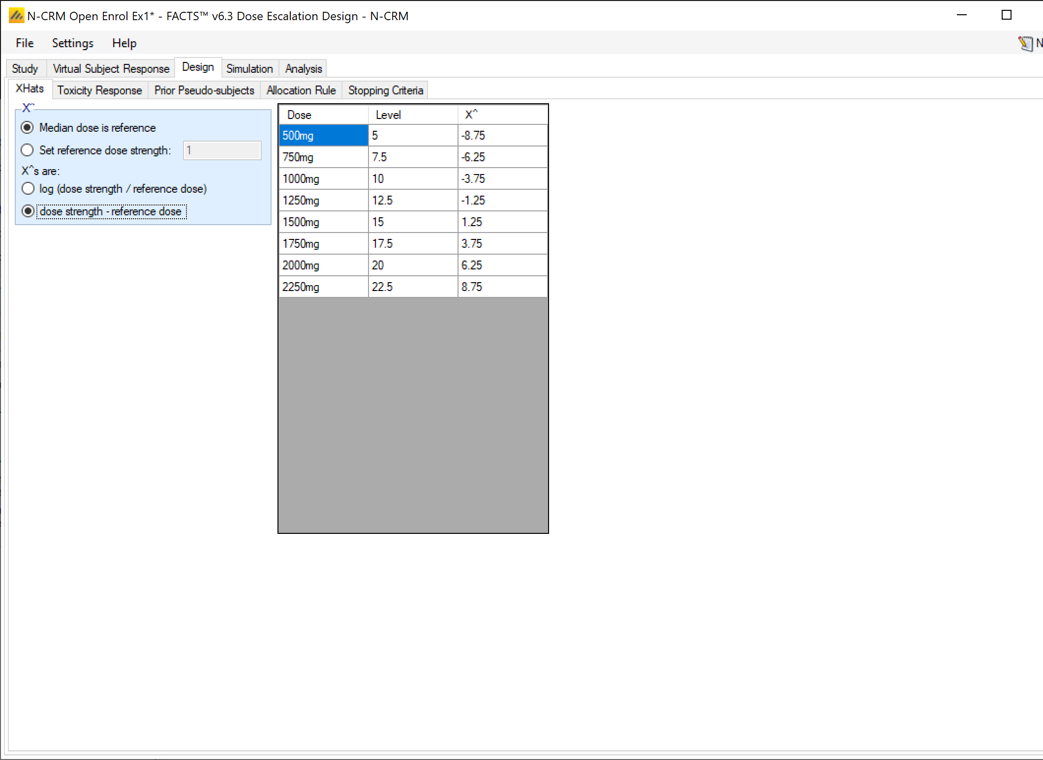
Where: \(\hat{x}_j = d_j - d^{\ast}\) or \(\hat{x}_j = ln(\frac{d_j}{d^{\ast}})\) and \(d^{\ast}\) is the reference dose, due to this notational convention \(\hat{x}̂\), these transformed dose strengths are referred to as the “X-Hats”.

Note that in either transformation, when \(d_j = d^{\ast}\), then \(p_j = \frac{e^{\alpha}}{1 + e^{\alpha}}\).

The prior distribution is a bivariate Normal distribution of \(\alpha\) and \(ln(\beta)\):

\[ \begin{bmatrix} \alpha \\ ln(\beta) \end{bmatrix} \sim N \left( \begin{bmatrix} \mu_{\alpha} \\ \mu_{ln(\beta)} \end{bmatrix}, \begin{bmatrix} \sigma_{\alpha}^2 & \rho \sigma_{\alpha} \sigma_{ln(\beta)} \\ \rho \sigma_{\alpha} \sigma_{ln(\beta)} & \sigma_{ln(\beta)}^2 \end{bmatrix} \right) \]

With the user supplying the mean and standard deviation of \(\alpha \ (\mu_{\alpha}, \sigma_{\alpha})\), and \(ln(\beta) \ (\mu_{ln(\beta)}, \sigma_{ln(\beta)})\) and the correlation coefficient \(\rho\).

The efficacy model is the same.

Extensions:

If there are two groups the toxicity or efficacy response of the second is modeled: \[ ln(\frac{p_j}{1-p_j}) = \alpha + a + \beta b \hat{x}_j \]
- Where \(a\) and \(ln(b)\) have their own bi-variate normal prior. Note that as the response of the second group is modelled as an offset from the first an informative prior can be used to limit how large the offset is.
- Optionally \(b\) can be fixed at 1, so the two groups are modelled with a common estimate of the slope (\(\beta\))
- Optionally a may be constrained to be +ve or -ve so that (if there is a common estimate of the slope) the estimate of the toxicity rate for the second group can be constrained being higher or lower than that of the first group.

To allow N-CRM to be used to simulate old CRM designs, an option to fix the value of Alpha is included (for both toxicity and efficacy), this option is not recommended for new designs. Fixing the alpha means that the response model has a fixed rate of response at the reference dose – in the old CRM designs in effect the reference dose was above the highest dose.

If the toxicity model is of an ordinal toxicity rate, the toxicity response model is:

\[ logit(Pr(Y \geq j | \hat{x})) = \alpha_j + \beta\hat{x} \]

for ordinal response \(j=2,3\) or \(j = 2,3,4\). The \(\alpha_2\) and \(\alpha_4\) have independent Normal priors and are constrained to be \(\alpha_2 > \alpha_3 > \alpha_4\). The \(\alpha_3\) is fitted with the BLRM and bivariate Normal prior as for dichotomous toxicity, or it may be given a fixed value.

Lastly both the toxicity and efficacy models can the adjusted to be asymptotic at limits inside the interval \([0,1]\). For example if the toxicity being observed has a ‘natural’ background rate then the minimum asymptote could be adjusted to this rate.

If the rate given by the BLRM is \(p’_j\) then the actual estimated rate is \(p_j\) adjusted to lie between \(p^{max}\) and \(p^{min}\) where:

\[ p_j = p’_j(p^{max} - p^{min}) + p^{min} \]

X-Hats

On this tab the user specifies the reference dose \(d^*\) for use in calculating the adjusted dose value (the “x-hat” values). The default value to use is Median dose is reference, this uses the median of the dose range for the reference dose, minimizing the correlation in the sampled values of \(\alpha\) and \(\beta\). Note though that when allocation is restricted to explicit doses it is also recommended that the value of the reference dose is not the same as an actual dose that can be used (at this dose \(\hat{x}\) will be 0 and the data on this dose can have undue weight on the estimate of \(\alpha\)).

Different reference doses can easily be used however – between the two doses thought most likely to be MTD, just below the lowest dose, just above the highest dose. The bi-variate Normal prior for \((\alpha, ln(\beta))\) will need to be recalibrated to take the change into account.

X-Hats are log(dose strength) allows the user to select between:

linear effective dose \(\hat{x}_j = d_j - d^*\)
\(log(\hat{x}_j) = ln(\frac{d_j}{d^*})\)

If you have entered linear dose strengths for the doses (1, 2, 3, 4, … or 100, 150, 200, 250, …) then use the linear effective dose. If however the dose strengths that have been entered are non-linear (12.5, 25, 50, 100, …) but expected to be roughly linear in effect, then use the log of the dose ratio.

Figure 40: Specifying the dose transformation - the “x-hats”.

The Pro’s & Con’s of using the median dose as the reference dose

The reason the median dose is recommended as the reference is that this minimizes the correlation in the fit of \(\alpha\) and \(ln(\beta)\), the parameters of the BLRM, and it maximises the flexibility of the fit of the model over the dose range.

However care needs to be taken that the prior on \(\alpha\) is not more restrictive than that on \(ln(\beta)\) in order to avoid a phenomena observed when preparing tutorials: observing “no toxicities” below the reference dose resulted in a model with increased probability of toxicity above the reference dose compared to observing a toxicity below the reference dose. For a given value of \(\alpha\), higher values of \(ln(\beta)\) correspond to lower toxicity below the reference dose – as the \(\hat{x}\)̂ values are -ve below the reference dose. The fitted curve thus “pivots” about the value of \(\alpha\) at the reference dose.

There are two solutions to this:

move the reference dose, which involves a choice between two options
1. moving it to the first dose or below (normally allowing a relatively constrained prior around a low value for \(\alpha\)),
2. or to the highest dose or above (with a relatively uninformative prior).
We have seen both solutions perform well against the chosen scenarios – but the choice needs checking and refining with a full range of scenarios that represent the full uncertainty in the true response.
or modify the priors on \(\alpha\) and \(ln(\beta)\) making the prior on \(\alpha\) less informative (in particular increase the probability of low values) and make the prior on \(ln(\beta)\) more informative (in particular lower the probability of high values less). Because the prior distribution on \(\beta\), is on \(ln(\beta)\), it is easy to make large values of \(\beta\) more probable than intended.

Toxicity Response

The parameters that can be specified on this page are:

The parameters of the bivariate Normal distribution for \(\alpha\) and \(ln(\beta)\). Specifying the mean and standard deviation of \(\alpha\) \((\mu_{\alpha}, \sigma_{\alpha})\), and \(ln(\beta)\) \((\mu_{ln(\beta)},\sigma_{ln(\beta)})\) and the correlation coefficient \(\rho\).
- If ordinal toxicity is being simulated, it is possible to model the ordinal toxicity, specifying the mean and standard deviation of \(\alpha_2\) and \(\alpha_4\). These priors are separate from the \(\alpha_3\) and \(ln(\beta)\) prior, there is no correlation term in the prior. There is the constraint in the model that \(\alpha_2 > \alpha_3 > \alpha_4\).
- Use fixed Alpha: the value of Alpha can be fixed to allow the N-CRM model to behave like the traditional CRM models. [Where \(\alpha\) was set to 3 and the reference dose is set above the top of the available dose range]

Rather than entering the priors directly, they can be derived based on indirect prior information or beliefs, see ‘Deriving the Prior’ below.

The Minimum and Maximum rates that the model is to be fitted too. The model fits the range \((0,1)\), asymptotically approaching each limit as the adjusted dose value tends to \(-\infty\) or \(+\infty\). By specifying an alternative minimum and maximum, inside the range \((0,1)\), the user can have the model scaled to fit data to fit event rates where the asymptotic rates are not \(0\) or \(1\). For instance if the event being observed has a non-zero background rate (probability of being observed in placebo treated subjects), then the model may fit better if the minimum is set to the lower limit of this expected rate. Similarly if, even at the most toxic dose the event being observed is only expected to effect a proportion of subjects, the model may fit better if the maximum is set to the upper limit of this expected rate.
If a control arm is present, the user can specify to have this modelled separately, and if so the user specifies the parameters for a prior Beta distribution – in terms of numbers of prior observations on control of subjects with and without a toxicity.
Group 2 priors: if a second ‘Group’ is being simulated – whether this is a subset of subjects, or a modified treatment that subjects can be randomized to, then the BLRM is jointly fitted to the responses for both groups, with group 2 having offsets \(a\) and \(b\) from the first group’s \(\alpha\) and \(\beta\). The priors for \(a\) and \(b\) can be full bivariate Normal or can use constraints such as \(b = 1\), or \(a > 0\) or \(a < 0\).

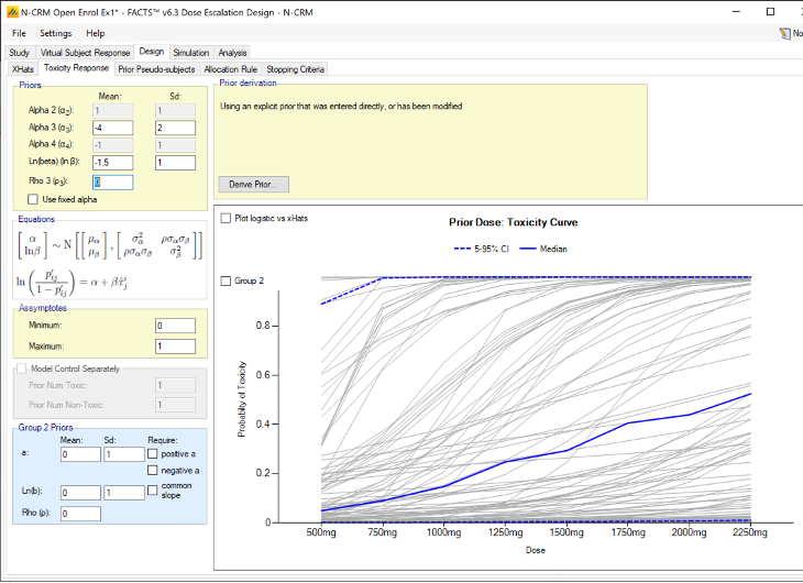
Deriving the prior

The priors of \(\alpha\) and \(ln(\beta)\), can be specified directly or derived in one of four ways. When entered explicitly, the user specifies the parameters of the prior bivariate-normal distribution for \(\alpha\) and \(ln(\beta)\): the means, standard deviations and the correlation term \(\rho\).

Alternatively, the user may click the ‘derive prior’ button and select from:

Quantiles at the lowest and highest dose: (based on the “uninformative prior” given in the paper (Neuenschwander, Branson, and Gsponer 2008), for details see this section) - the user specifies the probability of an unacceptable toxicity at the lowest dose, and the probability of under-dosing at the highest dose (0.1 for both is the default, and 0.05 for both is the value used in the paper). Optionally the probability that toxicity is less than the mid-point of the target toxicity band at the median dose can be specified. (Prior to FACTS 6.5 this third data point was not optional and constrained to be at the reference dose, but this had problems if the reference dose was not the media dose – it might also be the lowest dose for example).

Note this method does not work so well if the reference dose is outside the dose range.

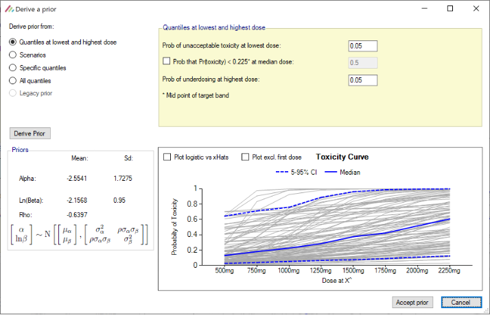
Figure 42
Scenarios: the model is fitted to each of the toxicity response scenarios (MLE), the parameters of the bivariate normal are then calculated from resulting set of pairs of values for \(\alpha\) and \(ln(\beta)\).

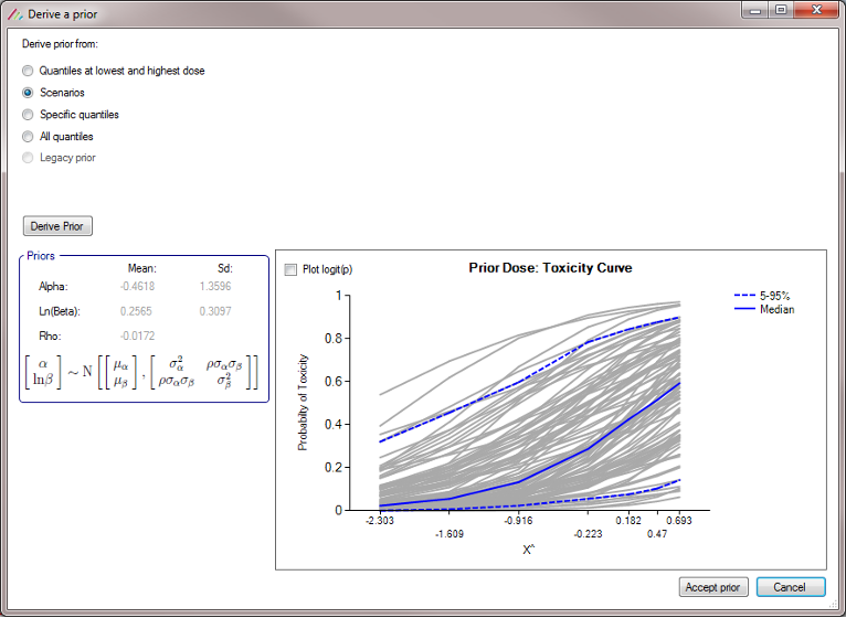
Figure 43
Specific quantiles: The user selects which doses and toxicity rates to provide an expectation – a prior probability that the toxicity rate on the dose will be the specified rate or less. At least 3 such expectations using at least 2 different doses strengths must be supplied. If a large number of specific quantiles are specified (e.g. reproducing the all quantiles method) the large number of different beta distributions sampled from, with the monotonicity constraint applied, results in losing too much variability. So this should only be used quantiles specified at 2-4 doses.

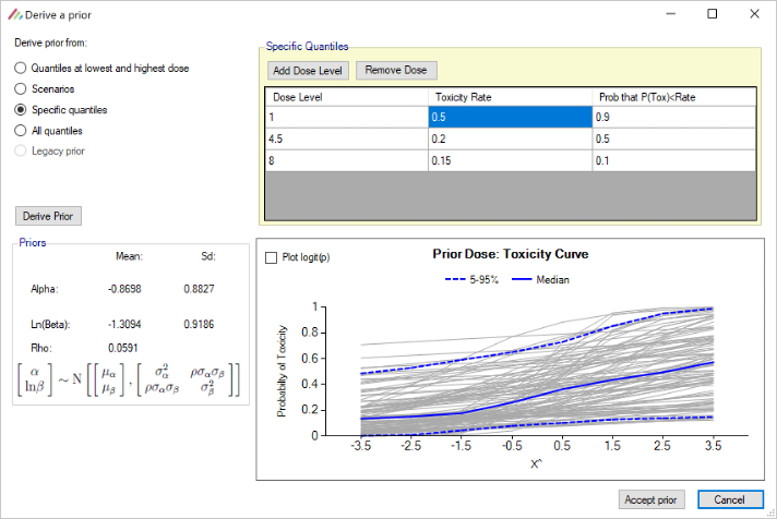
All quantiles: the user specifies the prior expected toxicity rate at the 2.5%, 50% and 97% quantiles for each dose. (Only available when using explicitly defined doses, not a continuous dose range). Note that using Create Prior with this option will require the facts file to be saved and for there to be at least one virtual subject response profile.

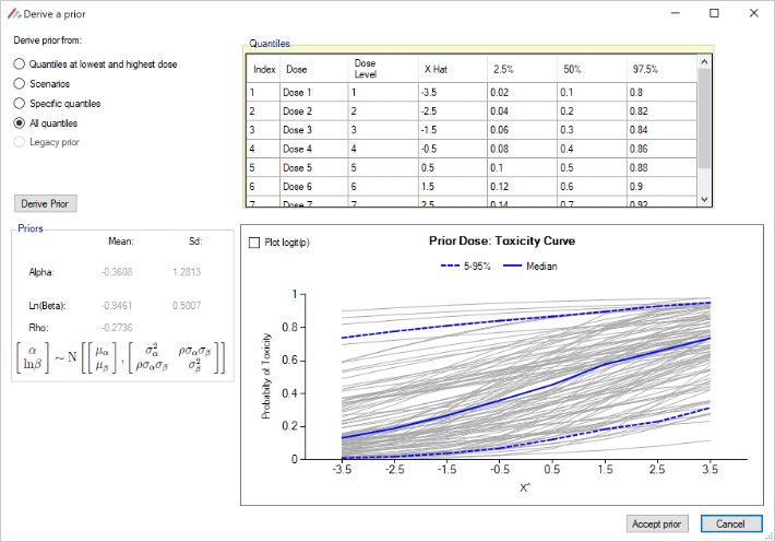
In all cases once prior values have been derived they are displayed along with a graph of 100 sampled curves from the prior. The user can accept the values, change derivation method, or cancel the derivation.

The plot of the samples can either be viewed as Pr(Tox) or Log-odds(Tox) vs relative dose (“x-hat”).

Derivation of the Prior from Quantiles

Derivation of the parameters of the bivariate Normal prior for \(\alpha\) and \(ln(\beta)\)) in the Quantiles at lowest and highest dose, Specific quantiles and All quantiles cases:

Minimally informative unimodal Beta distributions are fitted for each of the doses where a prior expectation of a toxicity has been specified. For doses where no prior expectation has been specified, the median expected toxicity rate are derived by assuming that the median expected toxicity is linear in log dose on the logit scale, and again a minimally informative unimodal Beta distribution is fitted with the same median.
Previously and following (Neuenschwander, Branson, and Gsponer 2008), the parameters of the bivariate Normal distribution were found using a stochastic fit to the prior expectations of toxicity, minimizing the error in the prior toxicity rates at the 2.5%, 50% and 97.5% quantiles. This is still used in the All quantiles and Legacy prior cases. However experience with this method with the standard priors (previously called “uninformative”) showed that it yielded priors with too little uncertainty in the \(ln(\beta)\)) and too high a value for the correlation parameter for many cases and certainly for the prior to be called “uninformative”.
Consequently, in the Quantiles at lowest and highest dose and Specific quantiles cases, the prior is now derived by sampling from the minimally informative unimodal Beta distributions, and fitting the model to each set of sampled toxicity rates. The parameters of the bivariate normal are then calculated from resulting set of pairs of values for \(\alpha\) and \(ln(\beta)\).

If a control arm has been included, it may be included in the model, or modelled separately using a beta-binomial model, the user specifies the prior values for the Beta distribution.

Derivation of the prior from the scenarios

In this screenshot, priors have been derived from the scenarios:

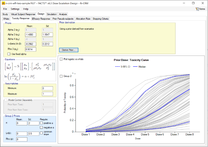
Figure 46: Design - Toxicity Response sub-tab (after prior derivation)

Clearly in this example the scenarios have a very high correlation between the toxicity at the reference dose (\(\alpha\)) and the log gradient (\(ln(\beta)\)) giving a high value for the correlation in the prior (\(\rho\)). As there are very few scenarios, and they didn’t include extreme cases, the SDs of the priors of parameters will be underestimated.

So In this instance we might round the prior means to 2 decimal places, double the SD of \(\alpha\), slightly increase the SD of \(ln(\beta)\) and reduce the correlation to 0.5.

However, it is much better to use Drive from Scenarios after entering a large number of varied and credible scenarios. Indeed is such a collection of scenarios exists, deriving the prior from the scenarios is the simplest approach and often very effective. Only if the performance in the simulations in some scenarios does the prior need re-visiting (usually to slightly increase the \(ln(\beta)\) SD and/or reduce the correlation).

We strongly recommend checking the performance of the prior across a wide range of scenarios, and of entering the reported derived values of the fitted prior as an explicit prior and then manually modifying them in the light of the model’s performance on the various scenarios.

Legacy prior methods

In old versions N-CRM (pre-FACTS 4.0) , the design could be left at the stage where the method of deriving the prior had been specified but the derivation postponed to the simulation stage. We now require that the derivation be performed first, this

Enables the actual prior that results from the derivation to be inspected
Makes simulation and recommendation faster, as the derivation is not repeated every time the design engine starts.

When opening a FACTS N-CRM file created using a pre-FACTS 4.0 version of FACTS, to continue to use the original prior, select “Derive prior”, and the derive prior window will display the old prior and allow an explicit prior to be derived from it using the now deprecated methods in the older versions of FACTS N-CRM.

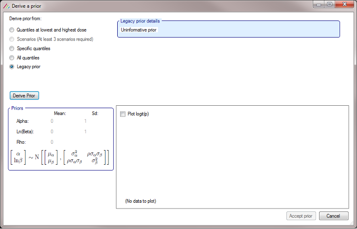
Figure 47: Derivation from a legacy prior

Efficacy Response

The Efficacy Response tab is displayed if an efficacy endpoint is included in the trial.

The Efficacy Response is specified separately from the Toxicity Response. The Toxicity and Efficacy models are completely separate except for the x-hat values for the transformed dose strengths, where a common set of values is used for both models. Note that the use of a common set of x-hats for both endpoints is a difference from FACTS bCRM, that means it may not be possible to exactly replicate a bCRM design in FACTS N-CRM, however we think that the additional features and options in FACTS N-CRM will make it possible to create an overall superior design in FACTS N-CRM.

The features available for specifying the Efficacy Response model are the same as the Toxicity Response model (see above) – with the exception that the Toxicity Response includes an option for modeling ordinal toxicity, there is no corresponding ordinal efficacy option.

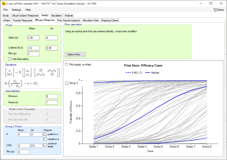
The same options for deriving the prior are available as for the Toxicity Response Model.

Prior Pseudo-subjects

This option allows “prior data” or “pseudo data” to be specified that will be included in every analysis. This is equivalent to the model being fitted with the parameter prior to this pseudo data and the resulting posterior being the new prior, but it is easier and quicker to include the pseudo subject with the real data and do one analysis.

The user selects which dose levels at which to include the data and specifies the number of pseudo/prior subjects/observations and the number of toxicities. These are allowed to be fractional, and observations can be at dose levels not being tested in the trial. In each analysis the observed data is augmented with this specified data and the parameters of the toxicity response estimated.

If there is an efficacy endpoint as well as toxicity endpoint, pseudo subject data is specified separately for the two endpoints (not surprisingly!). If the data is to be analyzed as “2 groups” pseudo subject data is also specified separately for the two groups.

The effect of this data on the prior can be visualized by the “Update Plot” function that estimates the parameters of the toxicity response and plots the curves of 100 samples drawn from the posterior estimates of the parameters of the model.

The plot of the samples can either be viewed as Pr(Tox) vs Dose Strength or Log-odds(Tox) vs relative dose (“x-hat”).

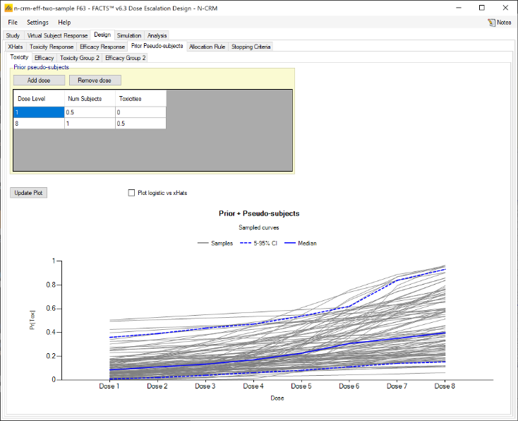
Figure 49: Specifying prior pseudo subjects

Example of effect of pseudo subjects on prior
Prior Only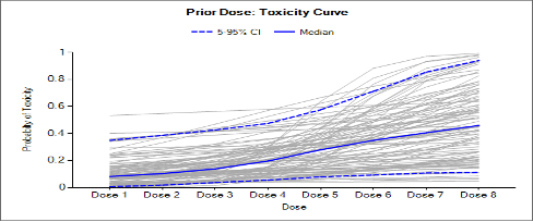
Prior plus 0.5/0 subjects toxicities on dose 1 and 1/0.5 on dose 8.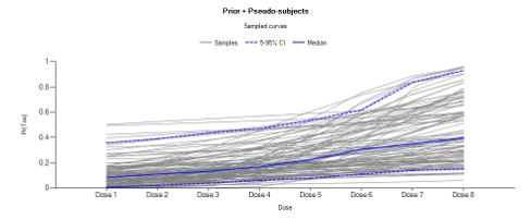
Prior plus 3/0 subjects / toxicities on dose 1 and 3/1.5 on dose 8.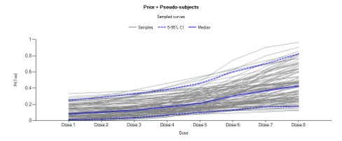

Allocation Rules

The Allocation Rule sub-tab is depicted below (Figure 50); it allows the user to select and set the parameters for the allocation rules.

There is an option to mimic the original Neuenschwander paper and rely on just the toxicity model and the overdose control to guide allocation – i.e. allocate to as close to the estimate of the MTD as we can limited only by the overdose control limits. This is “Use only overdose control”. Normally however we think the clinical will want to impose additional allocation rules.

The next dose allocated is a combination of the current target dose, and 2 possible maximum allocatable doses:

The target dose is the dose with the highest probability of being the target: the dose with the greatest estimated probability that its toxicity rate lies in the target toxicity band, or the dose nearest or highest below the MTD depending on the options selected on the Study > Toxicity tab.
The highest dose that meets the overdose criteria (if any): the highest dose that does not have a posterior probability that its toxicity rate lies in the excess & unacceptable toxicity bands or unacceptable toxicity bands above the threshold specified on the Study > Toxicity tab.
The current cleared dose and how far above that dose can be allocated to as defined by the specified allocation rules (if any).

The next dose to be allocated to is the lowest of these 3 doses.

It is possible to specify a “run-in” phase before this dose escalation phase applies. A run-in phase has a fixed sequence of doses and cohort sizes (typically smaller than the cohort size used in the escalation phase) and lasts up to the first observed toxicity or the end of the sequence of doses.

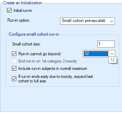
If the user selects to use an “Initial run-in” then there are 3 run-in types that can be selected from:

“Simple run” (the only type available before FACTS 6.3): cohorts are of a single size and the dose sequence up to the “Run-in cannot go beyond” dose (if specifed) is either:
- at every dose starting at the specified “initial dose” if explicit doses have been defined on the the Study > Treatment Arms tab,
- at the dose increment intervals defined in the allocation rules if finely spaced doses have been defined on the Study > Treatment Arm tab.
“Custom run-in” where the user specifies which doses are selected (leaving the “number of subjects” at a dose at 0 mans it is not selected) and at each dose how many subjects are allocated in the cohort at that dose.
Small cohort pre-escalation, cohorts are of a single size and the dose sequence follows the dose increment intervals defined in the allocation rules up to the “Run-in cannot go beyond” dose (if specifed).

“Simple run-in” and “Small cohort pre-escalation” the user specifies the “small cohort size” and there is an option to specify a top dose that the “Run-in cannot go beyond”.

For all run-in schemes there are options:

End run-in on 1st category 2 toxicity: The default for the simulation is to stop the run-in when the first full toxicity is observed, there is an option to instead stop when a lower grade toxicity is observed – a category 2 toxicity. If this option is selected, the simluation of virtual subjects is extended to include the simulation of category 2 tocxicity as well as category 3.
Include run-in subjects in overall maximum
When run-in ends expand last cohort to full size
- If this is not set then N-CRM model is applied and the next cohort is allocated as close to the target as possibly, restricted by the overdose restrictions and not allocating any higher than the dose reached in the run-in.
- If this option is set then last allocated small cohort is treated as the start of a full cohort and the remaining subjects are allocated at the same dose. The N-CRM model is then applied and the next cohort allocated according to the overdose restrictions and allocation rules. [Note it is possible that after observing no toxicities in the run-in or in the expanded cohort, that the overdose control will force a de-escalation in dose, depending on the priors for the model parameters and the overdose control limits]

If simulating 2 groups, and a run-in is specified, group 2 will only use a run-in if on the Study tab the option “Recruit Group 1 and Group 2 together” has been selected. Otherwise only group 1 will use the specified run-in, once group 2 starts it starts with the full cohort (or if open enrollment is being used, the full number of subjects to clear the dose). If using a run-in and recruiting groups 1 and 2 together then both use the same run-in rules, and both will stop on the first toxicity regardless of which group the toxicity occurs in.

If used, the Allocation rules have the effect of setting a Highest Allocatable Dose that specifies the highest dose level that can be allocated to by the allocation rules.

At the start the Highest Allocatable Dose is the user specified Starting dose level.
A dose is not ‘cleared’ until ‘The minimum cohorts on/near a dose before cleared’ have been allocated to it. If this is set to greater than one, then the specified number of cohorts must have been allocated to the current dose before it is ‘cleared’. Typically this parameter would be set > 1 when small cohort sizes are being used (such as 1 or 2 subjects per cohort) and/or when cohorts are assigned before a previous cohort’s results are available.

If using Open enrolment, this parameter is ’The minimum subjects on a dose before cleared’ and refers to the number of complete subjects.
The user can specify that Dose not cleared if proportion toxic on dose > and a maximum level of toxicity that can be tolerated for the current dose to be ‘cleatred’. This is of course somewhat of a ‘belt and braces’ approach – it being likely that the model would not want to increment if the proportion of toxicity is high, and indeed if an undesired behavior is observed in simulations, the behavior of the model and the effect of the prior should be investigated.
The user specifies whether the dose increment rules are to be specified in terms of the number of dose levels that can be incremented or in terms of the ratio by which the dose strength can be increased. If using “dose strength” it is up to the user to ensure that the specified ratio is sufficient to allow all doses to be reached. For example if in the dose range there is a dose of strength 100 and the next dose is of strength 200, then if any dose increment rule is specified that doesn’t allow the dose strength to at least double (using “ratio of dose strength” of less than 2) then the rule will prevent escalation from the 100 dose to the 200 dose.
The maximum amount the dose can be incremented can be specified in 3 ways:
- Single value: For all doses, once a dose has been cleared the next ‘highest allocatable dose’ is the dose above the cleared dose by the specified increment – either a number of dose levels or by a proportion of the dose strength.
- By total number of toxicities: With this rule the maximum dose increase allowed depends on the total number of toxicities that have been observed in the trial so far. The user specifies the maximum increment (in terms of the number of dose levels or the maximum proportional increase in dose strength) when no toxicities, one toxicity, or more than one toxicity has been observed.

Figure 9-5 Maximum dose increment varying by number of toxicities observed

Figure 51: Maximum dose increment varying by number of toxicities observed

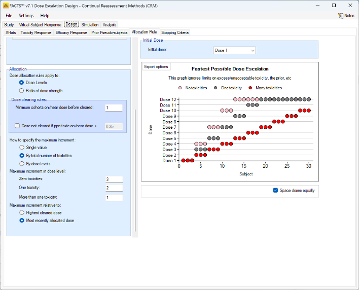
By dose levels: the maximal permitted increment is defined in terms of the number of dose levels or the proportional increase in dose strength that the dose can be increased, in up to 3 bands of dose strength. The user defines the upper and lower doses of the middle increment range, the lower range is then from the lowest up to this band and the upper band is from the top of the middle band to the highest dose. The user then specifies the maximum number of dose levels or the maximum proportional dose strength that can be incremented if the current dose is within each of these bands.

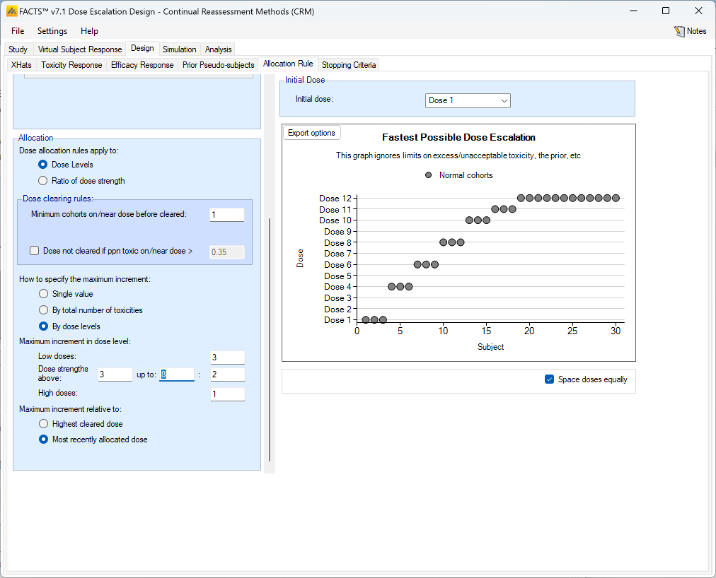
Figure 52: Maximum dose increment varying by dose level

If toxicities are observed that causes the N-CRM to allocate a dose below the current cleared dose, then there are two options for what happens to the current cleared dose:
- it is left unchanged and further increments are applied relative to the Highest cleared dose.
- it is reduced to the dose level selected by N-CRM, and further increments are applied relative to the Most recently allocated dose.
If a Control arm has been included, the user must specify the number of subjects per cohort to be allocated to Control. (The Control arm will never be the MTD and thus whole cohorts will never be assigned to it, so it must have a fixed number of subjects assigned from each cohort).

The “Fastest Possible Dose Escalation” graph shows the dose allocation permitted by the rules if no toxicities are observed. Or the graph can be changed to show the allocation if a toxicity occurs at a specific dose during the run-in.

If there are 2 groups and recruitment to the second group is delayed (either until the first group is complete, has reached a specific dose, or tested a specified number of subjects). Then starting dose for the second dose can be specified as

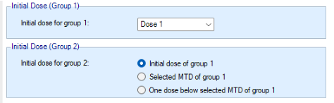
Figure 53: Design - Allocation Rule Initial Dose Second Group

Allocation rules when using a fine grained dose range

When a fine grained dose range is being used, the specification of the allocation rules change to accommodate the fact that the trial is no longer stepping up a few pre-defined dose levels. As with the explicit doses, the allocation rules work with the notion of a Currently Permitted Maximum Dose (CPMD).

At the start the highest allocatable dose is the user specified Starting dose strength.
A Run-in phase can be specified, this will always begin at the start dose and allocate ‘small cohorts’ following the maximum increment rules (this is different from when there are explicit doses – with explicit doses, the simple run-in simply allocates successive small cohorts to successive doses, ignoring the maximum permitted increment) for a simple run-in or small cohort pre-escalation, or the specified allocation pattern for a custom run-in, until the first toxicity is observed.
The degree of increment and specification of what counts as a ‘close’ dose, can be done either in Dose Strength or Ratio of dose strength.
A dose is not cleared until ’The minimum cohorts on a dose before incrementing’ have been allocated to it. Typically this parameter would be set > 1 when small cohort sizes are being used (such as 1 or 2 subjects per cohort) and/or when cohorts are assigned before a previous cohort’s results are available.
The user can specify that Dose not cleared if ppn toxic on/near dose > and a maximum level of toxicity that can be tolerated before the dose is cleared. This is of course somewhat of a ‘belt and braces’ approach – it being likely that the model would not want to increment if the proportion of toxicity is high, and indeed if an undesired behavior is observed in simulations, the behavior of the model and the effect of the prior should be investigated.
The Max ratio of dose strengths considered as near or Delta in dose strength considered as near defines a margin such that when evaluating whether a dose that has been allocated to counts as “cleared”, then cohorts allocated within that margin all count as being “on” the dose to allow incrementing.
The Maximum increment selected by option allows the user to specify varying maximum increments either dependent on the current cleared dose (Dose strength), or on the Total number of toxicities that have been observed, as follows:
- Single value: the amount by which the highest allocatable dose can be above the current cleared doses is constant throughout the trial. (This simple rule can work well when combined with overdose control. The two more complex rules are essentially trying to achieve the same thing as overdose control but are more simplistic and it may be confusing as to whether the allocation rule or overdose control is preventing escalation at any given moment).
- Total number of toxicities: the amount by which the highest allocatable dose is above the current cleared dose is specified separately for whether zero, one or two or more toxicities have been observed in the entire study.
- Dose strength: The user specifies:
  - the increment at low doses;
  - the increment at medium doses, along with the upper and lower dose strengths that define the bounds of what constitutes a ‘medium dose’; and
  - the increment at high doses.
If toxicities are observed that causes the N-CRM to allocate a dose below the current cleared dose, then there are two options for what happens to the current cleared dose:
- it is left unchanged and further increments are applied relative to the Highest cleared dose.
- it is reduced to the dose level selected by N-CRM, and further increments are applied relative to the Most recently cleared dose.
If a Control arm has been included, the user must specify the number of subjects per cohort to be allocated to Control. (The Control arm will never be the MTD and thus whole cohorts will never be assigned to it, so it must have a fixed number of subjects assigned from each cohort).

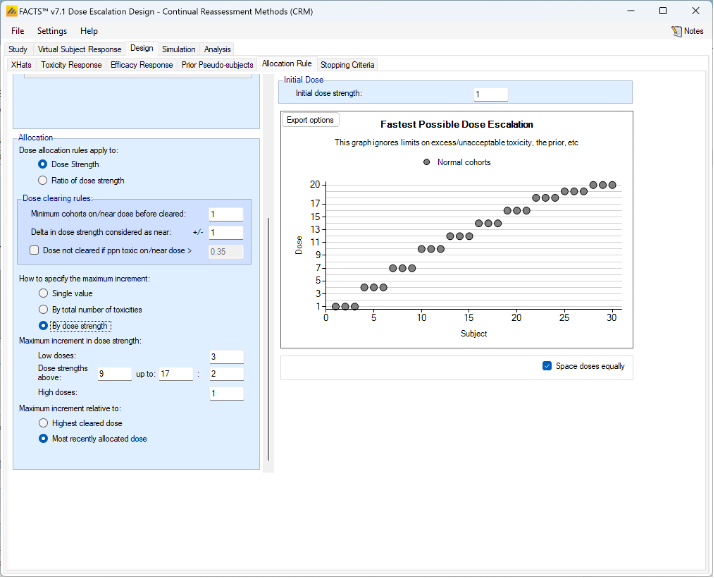
Figure 54: Allocation rules with a finely spaced doses

Backfill Allocation

If the trial is using open enrolment then “Backfill” allocation is an option. Backfilling is enabled on the Study > Study Info tab, where the maximum number of subjects that can be allocated when backfilling is specified.

Backfilling is the allocation of subjects to a dose below the current dose when the maximum number of subjects on the current dose without final results has been reached.

The Backfill Allocation tab allows detailed control of when backfilling can be used. The user specifies:

The maximum overall number of subjects that can be on a dose for backfilling to be allowed to that dose.
The maximum number of subjects that can be allocated to a dose by backfill.
The maximum number of dose levels below the current dose that can be used for backfilling (the highest that can be backfilled to will be used)
The lowest dose strength that can be backfilled to.
Whether or not the current escalation dose is a candidate for backfilling as long as the maximum number of subjects in their DLT period (set in the Study > Study Info tab) is not exceeded (also known as “frontfilling”).
If frontfilling is enabled, whether these subjects should count towards the backfill allocation cap or the regular study allocation cap (specified in the “Study/Study Info” tab).

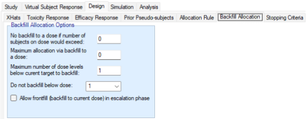
Stopping Criteria

The simulation will always stop when the maximum number of cohorts or subjects has been allocated.

The user may also specify that the study may stop early in terms of the amount of information that has been gathered about the target dose. In the N-CRM, the target dose can either be the Maximum Tolerated Dose or the “the allowed dose that has the highest posterior probability of having a toxicity rate in the Target Toxicity Band”; we use the label MTD (Maximum Target toxicity Dose) for this target dose too, for brevity and familiarity from previous CRM methods.

Note: if overdose limits have been set (see this section), then doses with posterior probabilities of having a toxicity rate in the Excess Toxicity or Unacceptable Toxicity bands that are greater than the specified thresholds, are disallowed for both dose allocation and selection as MTD.

To enable early stopping, the user must select “Rules for stopping trial early” there are then 2 rules which if selected are always “AND”ed together, and a further block of rules, the result of which (if specified) are “AND”ed with the first two rules. If more than one rule is selected within the block these may be either logically “AND”ed together or “OR”ed together to give the result of the rules in the block.

The two first standalone rules are:

If a “Required number of cohorts/subjects near MTD” rule is set then the trial will only stop early if at least this number of cohorts or subject has been allocated to the MTD dose or nearby doses. In the box above the “Count as MYD doses differing from MTD by less than or equal” allows how far away a dose can be and for cohorts/subjects on those doses to count towards this total. This can be set to 0 to count only cohorts/subjects on the MTD. It is provided for when fine grain dosing or a large number of explicit doses have been specified. If specified this rule this must always be met along with any other rules set for the trial to stop early.
If a “Minimum number of cohorts/subjects accrued” has been set then this specifies a lower limit on the sample size before early stopping is allowed. It is provided to allow a higher number of subjects on the MTD if one of the first doses appears to be the MTD. If specified this rule this must always be met along with any other rules set for the trial to stop early.

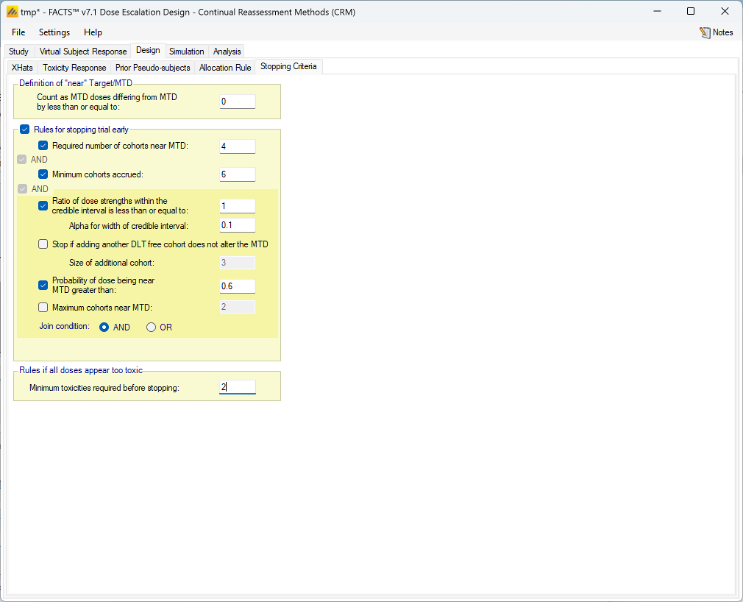
Figure 56: Design - Stopping Criteria sub tab

The available stopping rules are:

Required number of cohorts/subjects on/near MTD: Once the specified number of cohorts has been allocated to the dose currently determined to be the MTD, the trial may stop.
- This limit is defined in subjects if open enrollment rather than cohort enrolment is being used.
- The required number of cohorts/subjects can be “near” (rather than “on”) the MTD if a “Count as MTD” interval is defined. This interval is either defined by an interval of “dose strength” using the dose strengths defined on the Study > Treatment Arms tab, or by an interval of “dose strength ratios”. Which is used will correspond to the Selection for “Dose allocation rules apply to” on the Allocation Rules tab. A difference of 0, or factor of 1 can be used to only count cohorts/subjects actually on the selected MTD dose.
- If open enrolment is being used, there is an option to only pause accrual not stop it when the stopping rules have been met, in case the final results of any subjects that were not complete at the time the stopping rules were met cause the rules to be no longer met (for example by having results that change the dose estimated to be the MTD). If this option is selected then the stopping rules are re-assessed when all the current subjects are complete and the trial resumed if the rules are no longer met. Note this option is not required for cohort enrolment as stopping rules are only evaluated between cohorts.
Minimum cohorts/subjects accrued: this rule ensures that a minimum overall number of cohorts have been tested before the trial is allowed to stop. It makes no sense to use this rule on its own (it would effectively just lower the overall study cap) it should only be used in conjunction with other stopping rules.
- This limit is defined in subjects if open enrollment rather than cohort enrolment is being used.
The Additional Stopping Rules:
- Range/Ratio of dose strengths within the credible interval is less than or equal to: This is only enabled if on the Study > Study Info tab, the Type of Target has been set to “Target a single dose”. In this case the credible interval of the dose range that might contain the MTD is calculated, and this option allows the user to specify the width of the credible interval in “dose strength” to consider. How this works is a little counter intuitive: in each MCMC sample the engine determines which dose is the MTD and each doses’ Pr(MTD) is the proportion of the samples it was the MTD. The engine then calculates the minimum range of dose strengths required so that the sum of Pr(MTD) of the doses in the range exceeds 1 – Alpha. (So if a single dose has Pr(MTD) > 1-Alpha, the CI has zero width). If the xhats are log(dose strength) then the minimum range of log(dose strength) is found and exp() of this range returned.
  - The stopping rule is met if the width of the CI returned is less than that specified by the user.
  - If fine grain dosing is being used then the width of the target credible interval is defined as a dose strength ratio rather than a number of doses.
- Stop if adding another DLT free cohort does not alter the MTD: this rule is evaluated by analyzing the existing data supplemented by an additional cohort of a specified size where all the responses are no-toxicity; if this results in no change in selection of MTD then this stopping rule is met. If the study is using Open Enrolment, the user additionally specifies the size of the ‘virtual’ cohort to use.
- Probability of dose being in the target band greater than: in order to stop, the MTD’s posterior probability that its toxicity rate lies in the Target Toxicity band must be at or above the required threshold.
- Maximum Cohorts/Subjects near MTD: this option is supplied for use if the additional stopping rules are being OR’d together. (When they are AND’d together it simply functions the same way as the “Required Cohorts on MTD and stopping will not occur until the higher of the two targets is met).
- Join condition: if more than one additional stopping rule is selected, whether only any one of them needs to be met for the trial to be able to stop (Join condition = “OR”), of if all of the selected rules need to be met for the trial to be able to stop (Join condition = “AND”).

The study will also be stopped if there are no allowed doses by the overdose rules. However this can occur early in the study if a toxicity is observed in the first or second cohort. It is likely that in practice the clinical team would override the design stopping the study. Whilst it is difficult to fully represent the team’s decision making, a simple rule is included that is intended to approximate it:

Minimum toxicities required before stopping: This allows a requirement to be specified to observe a ‘minimum number of toxicities’ before the trial stops. If no doses are allowed by the overdosing rules, cohorts are assigned to the lowest dose until the minimum number of toxicities are observed, the stopping rules are met, or doses become allowable again after the model is updated after seeing no toxicities.

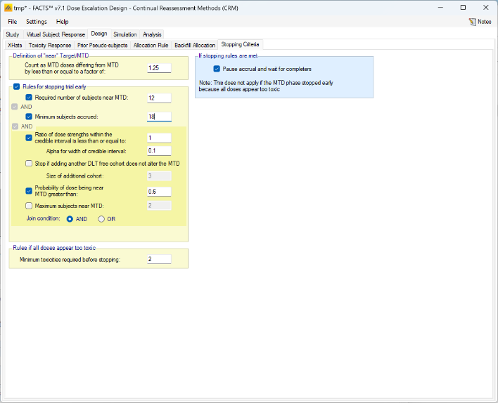
Figure 57: Stopping Criteria tab with open enrolment and finely spaced doses

If an additional efficacy endpoint is used, the MTD stopping criteria refer to when the trial jumps from assigning subjects with the aim of finding the MTD (“MTD phase”) to assigning subjects with the aim of finding the MED (“MED phase”). In the MED phase, it is possible that because of new data being observed, the MTD stopping rules are no longer met and the trial switches back to the MTD phase. A new stopping rule for the MTD phase is added, “Maximum subjects used to determine the MTD”. After this number of subjects has been enrolled, the trial switches from MTD to MED phase and there is no going back.

In the MED phase, there are several rules for stopping early (i.e. before the maximum sample size of the trial):

Maximum cohorts/subjects on MED. This behaves analogous to Required number of cohorts/subjects on/near MTD in the MTD stopping rules, with the exception of not using a concept of “near” doses.
Number of doses within the credible interval is less than or equal to with the sub-option Alpha for width of credible interval. This behaves analogous to Range/Ratio of dose strengths within the credible interval is less than or equal to in the MTD stopping rules.
Probability of dose being MED greater than. This behaves analogous to Probability of dose being in the target band greater than in the MTD stopping rules.

A special case arises when the MED estimate is larger than the MTD estimate. If that is the case, subjects are allocated to MTD or the highest cleared dose (whatever is smaller) even in the MED phase. The option “If MED > MTD: Continue until subjects near MTD reach” specifies how many subjects should be assigned to MTD in the MED phase before stopping the trial (and therefore giving up hope that the MED is a safe dose).

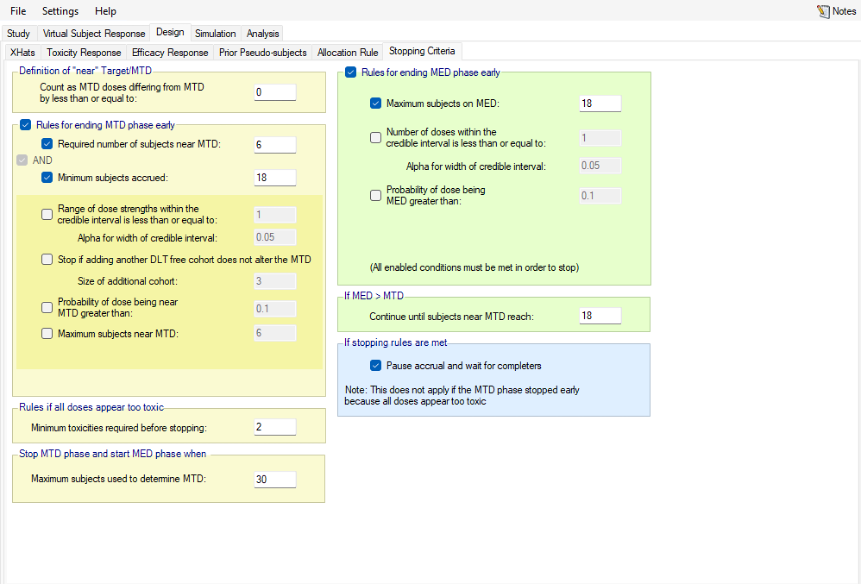
Figure 58: Stopping Criteria tab with open enrolment and both a toxicity and efficacy endpoint

Simulation

The Simulation tab allows the user to execute simulations for each of the scenarios specified for the study. The user may choose the number of simulations, whether to execute locally or on the Grid, and modify the random number seeds, Figure 59.

If completed results are available, the actual number of simulations run for each scenario is reported in one of the first columns of the results table. The value displayed in the “Number of Simulations” control is the number of simulations that will be run if the user clicks on the ‘Simulate’ button.

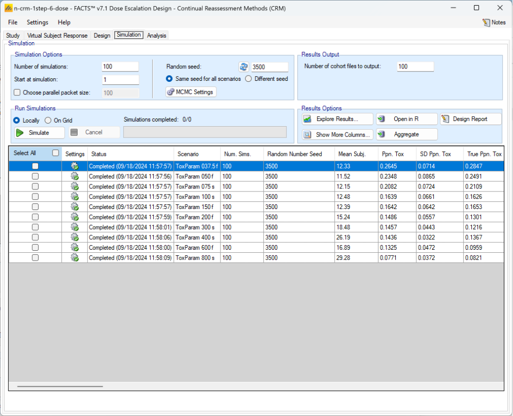
N.B. FACTS uses Markov Chain Monte Carlo methods in the generation of simulated patient response data and trial results. In order to exactly reproduce a statistical set of results, it is necessary to start the Markov Chain from an identical “Random Seed”. The initial random seed for FACTS simulations is set from the simulation tab, the first thing that FACTS does is to draw the random number seeds to use at the start of each simulation. It is possible to re-run a specific simulation, for example to have more detailed output files generated, by specifying ‘start at simulation’.

Say the 999th simulation out of a set displayed some unusual behavior, in order to understand why, one might want to see the individual interim analyses for that simulation (the “weeks” file), the sampled subject results for that simulation (the “Subjects” files) and possibly even the MCMC samples from the analyses in that simulation. You can save the .facts file with a slightly different name (to preserve the existing simulation results), then run 1 simulation of the specific scenario, specifying that the simulations start at simulation 999 and that at least 1 weeks file, 1 subjects file and the MCMC samples file (see the “MCMC settings” dialog) are output.

Even a small change in the random seed will produce different simulation results.

By default he same random number seed is used at the start of the simulation of each scenario. If two identical scenarios are specified then identical simulation results will be obtained. The same may happen if scenarios or designs only differ in ways that have no impact on the trials being simulated, for instance designs that have no adaptation, or scenarios that don’t trigger any adaptation (e.g. none of the simulations stop early). To avoid this possible artificial correlation in results across scenarios, select the “Different seed” option.

The user can specify:

the number of simulations for which ‘Cohorts’ files are written. ‘Cohorts’ files record the data, analysis and recommendation at each interim (after each cohort).
The parallelization packet size, this allows simulation jobs to be split into runs of no-more than the specified number of trials to simulate. If more simulations of a scenario are requested than can be done in one packet, the simulations are started as the requisite number of packets and the results combined and summarized when they are all complete – so the final results files look just as though all the simulations were run as one job or packet. When running simulations on the local machine FACTS enterprise version will process as many packets in parallel as there are execution threads on the local machine. The overhead of packetization is quite low so a packet size of 10 to 100 can help speed up the overall simulation process – threads used to simulate scenarios that finish quicker can pick up packets for scenarios that take longer, if the number of scenarios is no directly divisible by the number of threads packetization uses all threads until the last few packets have to be run and finally the “Simulations complete” figure can be updated at the end of each packet, so the smaller the packet the better FACTS can report the overall progress.

Simulation with Variants

The only difference that specifying design variants (see this section) introduces is to create additional scenarios – one for each Virtual Subject Response (VSR) profile for each variant. For example if there were 5 VSR profiles and then 4 variants (different numbers of maximum cohorts) specified then would now be 20 scenarios in total. The scenario names have “_Var1”, “_Var2”, … appended to them. Once simulations have been run and the .facts file has been saved and re-opened the scenarios are listed in alphabetical order.

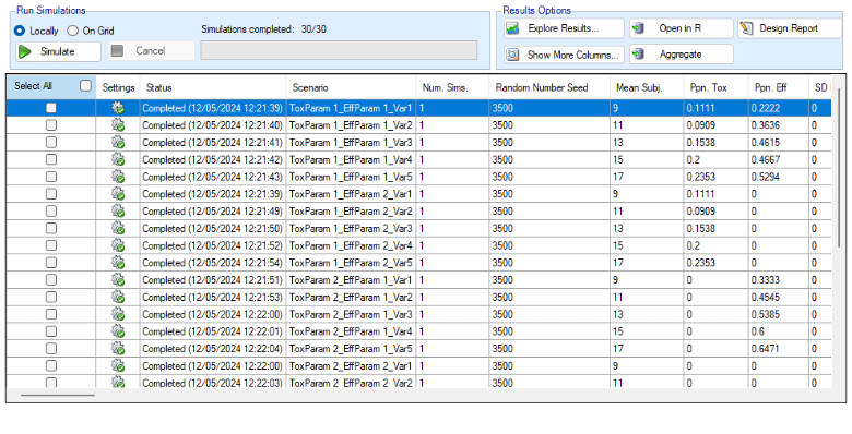
Figure 60: Simulation tab showing variants

To run simulations

Click in the check box in each of the rows corresponding the to the scenarios to be run. FACTS displays a row for each possible combination of the ‘profiles’ that have been specified: - baseline response, dose response, longitudinal response, accrual rate and dropout rate. Or simply click on “Select All”.

Then click on the “Simulate” button.

During simulation, the user may not modify any parameters on any other tab of the application. This safeguard ensures that the simulation results reflect the parameters specified in the user interface.

When simulations are started, FACTS saves all the study parameters, and when the simulations are complete all the simulation results are saved in results files in a “_results” folder in the same directory as the “.facts” file. Within the “_results” folder there will be a sub-folder that holds the results for each scenario.

How many simulations to run?

After first entering a design it is worth running just a small number of simulations such as 10 to check that the scenarios and design have been entered correctly. If all 10 simulations of a ‘null’ scenario are successful, or all 10 simulations of what was intended to be an effective drug scenario are futile, it is likely there has been a mistake or misunderstanding in the specification of the scenarios or the final evaluation or early stopping criteria.
Once the design and scenarios look broadly correct, it is usually worth quickly collecting rough estimates of the operating characteristics using around 100 simulations for each scenario. 100 simulations is enough to spot designs having very poor operating characteristics such as very high type-1 error, very poor power, a strong tendency to stop early for the wrong reason, or poor probability of selecting the correct target. 100 simulations is also usually sufficient to spot problems with the data analysis such as poor model fits and significant bias in the posterior estimates.
Typically 1,000 simulations of each scenario of interest is required to get estimates of the operating characteristics precise enough to compare designs and tune the parameters. (Very roughly rates of 5% (such as type-1 error) can be estimated to about +/-1.5% and rates of around 80% (such as power) estimated +/- 2.5%)
Finally around 10,000 simulations of the scenarios of interest is required to give confidence in operating characteristics of a design and possibly to select between the final shortlisted designs (Approximately rates of 5% can be estimated to about +/-0.5% and rates of around 80% estimated +/- 1%). This degree of accuracy usually unnecessary for dose escalation designs.

There may be many operating characteristics need to be compared over a number of scenarios, such as expected sample size, type-1 error, power, probability of selecting a good dose as the target and quality of estimation of the dose-response.

However frequently these will be compared over a range of scenarios, it may not be necessary to run very large number of simulations for each scenario if a design shows a consistent advantage on the key operating characteristics over the majority of the scenarios.

Simulation results

In the main screen the summary results that are usually of principal interest are displayed, the results summarised by scenario.

Show other columns: Allows the user to open additional windows on the simulation results, the windows available are:
- Open Results Folder: Opens the windows “File Explorer” tool in the results folder of the currently selected scenario. This makes it very easy to locate and open results files.
- Copy to Clipboard: will copy the values displayed in the summary to the clipboard as “CSV” data, enabling it to be pasted straight into a spreadsheet.
- All: A window containing all the summary results columns
- Highlights: a separate window with the results shown on the main tab
- Allocation, Observed: summary results of the number of subjects allocated, the number allocated to each dose, the number of toxicities observed and the number of toxicities observed per dose
- Fitted toxicity: summary results of the estimates of the model parameters and the dose-toxicity.
- Pr(MTD) etc: summary results of the posterior probabilities of the properties of interest
- Simulation Results: a window displaying the individual simulation results for each simulation of the currently selected scenario
Explore Results: offers three options:
- “Show Per Scenario Highlighted Scenario Graphs” that shows the graph of the simulation results for a specific scenario (see Section 12 below for a description of these graphs)
- “Show Across Scenario Graphs” that displays a trellis plot of summary graphs for each variant and each scenario (see Section 13 below for a description of these graphs).
- “Compare Scenarios in AIRSHIP” to open the simulation results in R with the AIRSHIP R-shiny graphing app. See the AIRSHIP User Guide for details.
Aggregate: opens a control that allows the user create aggregated results files from all the scenarios. The user can select which scenarios to include, and whether the results should be pivoted by dose. The resulting files are stored in the simulation results folder.
Open in R: If aggregated files have been created then clicking this button on the simulations tab will open control that allows the user to select which aggregations to load into data frames as R is opened. Otherwise it will offer to open R using the files in the currently selected scenario.
Design Report: it uses an R script and R libraries to generate a MS Word document describing the design. See the FACTS Design Report User Guide for details of what R packages need installing, how FACTS needs configuring to use the correct R instance, how the generate_report() function is run, and where the resulting report can be found.

Right Click Menu: right clicking the mouse on a row of results in the simulation tab brings up a ‘local’ menu of options corresponding to the above options that can be reached from the buttons, in what is sometimes a more ergonomic manner.

MCMC Settings

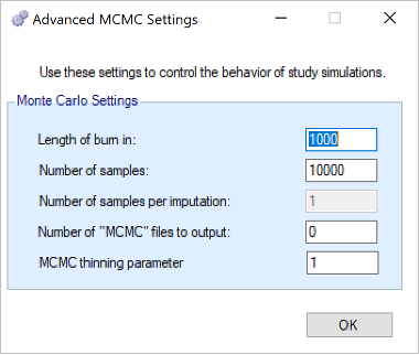
The first two values specify two standard MCMC parameters –

The length of burn-in is the number of the initial iterations whose results are discarded, to allow the sampled values to settle down.
The number of samples is the number of subsequent iterations whose results are recorded in order to give posterior estimates of the values of interest (in this case α and β).

The Number of samples per imputation value only applies to analyses using imputed data from a longitudinal model and is irrelevant for N-CRM, hence it is greyed out.

If the Number of MCMC files to output value is set to N, where N > 0, then all the sampled values at each interim in the first N simulations are output, allowing the user to check convergence.

The MCMC output thinning parameter can be used to reduce the amount of data output to the MCMC file. It does not reduce the amount of MCMC samples used within the model fitting.

To obtain the MCMC sampled values for a particular simulation, keep the same Random number seed and use Start at simulation to specify the simulation in question and run just 1 simulation.

FACTS Grid Simulation Settings

If you have access to a computational grid, you may choose to have your simulations run on the grid instead of running them locally. This frees your computer from the computationally intensive task of simulating so you can continue other work or even shutdown your PC or laptop. In order to run simulations on the grid, it must first be configured, this is normally done via a configuration file supplied with the FACTS installation by the IT group responsible for the FACTS installation.

Detailed Simulation Results

After simulation has completed and simulation results have been loaded, the user may examine detailed results for any scenario with simulation data in the table by double-clicking on the row. A separate window (as in Figure 62) will reveal more detailed results about the simulation.

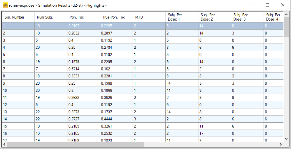
Right-clicking on a row displays a context menu from which the user can view other columns (the default are the “highlihgts” columns) and also view the corresponding cohort results:

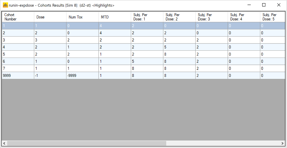
Figure 63: Cohort Results for a particular simulation

Right clicking on the cohort results, displays a context menu from which the user can view other columns (the default are the “highlights” columns).

Aggregation

Aggregation combines the csv output from multiple scenarios into fewer csv files. The Aggregate… button displays a dialog which allows the user to select what to aggregate.

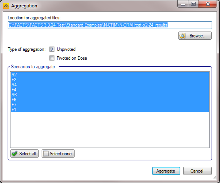
The default location for the aggregated files is the results directory for the study, but this can be changed.

Aggregation may be performed with or without pivoting on group, or both.

Unpivoted files will have one row for each row in the original files.
In pivoted files each original row will be split into one row per dose, plus two extra rows for ‘below lowest’ and ‘above highest’.
- Where there is a group of columns for each dose, they will be turned into a single column with each value on a new row.
- If there is no value for the below lowest or above highest rows, they will be left blank.
- Values in columns that are independent of group will be repeated on each row.

The default is to aggregate all scenarios, but any combination may be selected.

Pressing “Aggregate” generates the aggregated files.

Each type of csv file is aggregated into a separate csv file whose name begins agg_ or agg_pivot_, so agg_summary.csv will contain the rows from each of the summary.csv files, unpivoted. cohortsNNN.csv files are aggregated into a single agg_[pivot_]cohorts.csv file. Doses.csv is identical for all scenarios and so is not aggregated.

Each aggregated file begins with the following extra columns, followed by the columns from the original csv file:

Column Name	Comments
Scenario ID	Index of the scenario
Toxicity Profile	A series of columns containing the names of the various profiles used to construct the scenario. Columns that are never used are omitted (e.g External Subjects Profile if there are no external scenarios)
External Subjects Profile	A series of columns containing the names of the various profiles used to construct the scenario. Columns that are never used are omitted (e.g External Subjects Profile if there are no external scenarios)
Agg Timestamp	Date and time when aggregation was performed
Sim	Simulation number. Only present in the cohorts file.
Dose	Only present if pivoted

Design Report

This button becomes enabled once there are simulation results, it uses an R script and R libraries to generate a MS Word document describing the design.

See the FACTS Design Report User Guide for details of what R packages need installing, how FACTS needs configuring to use the correct R instance, how the generate_report() function is run, and where the resulting report can be found.

The Summary Results Columns

Results when 2 groups have been simulated

When 2 groups have been simulated, the results displayed on the Simulation tab and all the directly viewable summary tables under the “Show other columns” button are from Group 1.

To see the results from Group 2 you need to first display the Group 2 highlights – either by selecting “Group 2” on the “Show other columns” menu or after right clocking on a row of results.

Once the Group 2 “highlights” results are being displayed, the other sets of summary results can be viewed by right clicking on a row of results in the Group 2 “hightlights” window.

Highlights

These are the columns displayed on the simulations tab after simulations are completed, the can also be displayed in the separate “Highlights” results window.

Column Title	Number of columns	Description
Select	1	Not an output column, this column contains check box to allow the user to select which scenario to simulate. The ‘Select All’ button causes them all to be checked.
Settings	1	Displays an icon showing the status of the simulation results.
Status	1	This column reports on the current status of simulations: Completed, Running, No Results, Out of date, Error. It is updated automatically.
Scenario	1	This is the name of the scenario simulated. If only toxicity has been simulated this is simply the name of the Toxicity response profile to be simulated, if both efficacy and toxicity have been simulated, it is formed from the concatenation of the toxicity response profile name and the efficacy response profile name.
Num Sims	1	The number of simulations that were run to produce the displayed results.
Random Number Seed	1	Base random number seed used to perform the simulations.
Mean Subj.	1	This is the mean (over the simulations) of the number of subjects recruited in this scenario.
Ppn. Toxic	1	This is the average proportion of the subjects recruited that experienced a toxicity in this scenario.
Ppn. Eff	1	Included if efficacy is being simulated. This is the average proportion of the subjects recruited that experienced efficacy in this scenario.
SD Ppn. Toxic	1	This is the standard deviation of the proportion of toxicity across the simulations.
SD Ppn Eff	1	Included if efficacy is being simulated. This is the standard deviation of the proportion of efficacy across the simulations
True Ppn. Toxicity	1	This is the average true probability of toxicity over the simulations. The ‘true probability of toxicity’ in a simulated trial is the average of the probabilities of toxicity all the subjects are exposed to, given the toxicity response profile that we are simulating from.
True Ppn. Eff	1	Included if efficacy is being simulated. This is the average true probability of efficacy over the simulations.
MTD Selection: <dose>	One per dose	For each dose, this is proportion of the simulations where it was selected as the “MTD” at the end of the study. In CRM this is the minimum of: 1) the dose with the highest posterior probability of having a toxicity rate in the ‘Acceptable’ band and 2) the highest cleared dose. If limits on “excess” or “unacceptable” toxicity have been specified, then doses with posterior probabilities above these limits are excluded from being chosen as MTD. (Note this is different from the calculation of MTD used in Neuenschwander, Branson, and Gsponer (2008) where doses with posterior probabilities above these limits were not excluded from being selected as MTD.)
MED Selection: <dose>	One per dose	Included if efficacy is being simulated. For each dose, this is proportion of the simulations where it was selected as the “MED” at the end of the study. This is the dose with the highest posterior probability of being the dose that is the ‘highest dose below’ / ‘nearest’ / ‘lowest dose above’ (as specified on the Study > Effiacy tab) to the target efficacy rate.
Mean Duration	1	The mean (over the simulations) of the duration in weeks of the simulated trials.
SD Duration	1	The standard deviation over the simulations of the duration in weeks of the simulated trials.
Mean Lost	1	If the trial uses open enrollment, this is the number of subjects that could not be allocated a dose because the number of subjects treated but not yet complete had reached the specified “Maximum subjects without final result” limit. Otherwise the value is 0.
SD Lost	1	The standard deviation over the simulations of the number of subjects lost.
Ppn(All Tox)	1	The proportion of the simulations that stopped because all doses were too toxic.
Ppn(early Success)	1	The proportion of the simulations that stopped because sufficient stopping rules were met before the maximum number of cohorts had been treated.
Ppn(Cap)	1	The proportion of the simulations that stopped because the maximum number of cohorts had been treated.
Ppn MTD Under	1	The proportion of the simulations where true toxicity rate of the selected MTD dose lay in the “Underdosing” toxicity range.
Ppn MTD Target	1	The proportion of the simulations where true toxicity rate of the selected MTD dose lay in the “Target” toxicity range.
Ppn MTD Excess	1	The proportion of the simulations where true toxicity rate of the selected MTD dose lay in the “Excess” toxicity range.
Ppn MTD Unacc	1	The proportion of the simulations where true toxicity rate of the selected MTD dose lay in the “Unacceptable” toxicity range.
Ppn Correct Under	1	The proportion of the doses across all the simulations that were correctly identified as being in the “Underdosing” range. This will be 0 if none of the doses in that scenario had a true toxicity that fell in that range.
Ppn Correct Target	1	The proportion of the doses across all the simulations that were correctly identified as being in the “Target” range. This will be 0 if none of the doses in that scenario had a true toxicity that fell in that range.
Ppn Correct Excess+Unacc	1	The proportion of the doses across all the simulations that were correctly identified as being in the “Excess” or “Unacceptable” ranges. This will be 0 if none of the doses in that scenario had a true toxicity that fell in those ranges.
Ppn MED Under	1	Included if efficacy is being simulated. This is the proportion of the times the selected Minimum Efficacious Dose’s true efficacy rate was the target rate or less. (Note if the scenario contains a dose whose simulated true efficacy rate is exactly the minimum target rate selections of this dose will count as both MED Under AND Med Over))
Ppn MED Over	1	Included if efficacy is being simulated. This is the proportion of the times the selected Minimum Efficacious Dose’s true efficacy rate was the target rate or more. (Note if the scenario contains a dose whose simulated true efficacy rate is exactly the minimum target rate selections of this dose will count as both MED Under AND Med Over)

Allocations, Observed

Column Title	Number of columns	Description
Scenario	1	This is the name of the scenario simulated. If only toxicity has been simulated this is simply the name of the Toxicity response profile to be simulated, if both efficacy and toxicity have been simulated, it is formed from the concatenation of the toxicity response profile name and the efficacy response profile name.
Mean Subj.	1	This is the mean (over the simulations) of the number of subjects recruited in this scenario.
Ppn. Toxic	1	This is the average proportion of the subjects recruited that experienced a toxicity in this scenario.
Ppn. Eff	1	Included if efficacy is being simulated. This is the average proportion of the subjects recruited that experienced efficacy in this scenario.
SD Ppn. Toxic	1	This is the standard deviation of the proportion of toxicity across the simulations,
SD Ppn Eff	1	Included if efficacy is being simulated. This is the standard deviation of the proportion of efficacy across the simulations
True Ppn. Toxicity	1	This is the average true probability of toxicity over the simulations. The ‘true probability of toxicity’ in a simulated trial is the average of the probabilities of toxicity all the subjects are exposed to, given the toxicity response profile that we are simulating from.
True Ppn. Eff	1	Included if efficacy is being simulated. This is the average true probability of efficacy over the simulations.
Num Phase 1	1	Included if efficacy is being simulated. This is the mean (over the simulations) of the number of subjects recruited in the first phase (up to the MTD stopping criteria being met) in this scenario.
Subj. Per Dose: <dose>	One per dose	This is the mean (over the simulations) of the number of subjects assigned to each dose.
SD Subjects: <dose>	One per dose	This is the standard deviation of the number of subjects assigned to each dose across the simulations.
Cat 2 Tox per Dose: <dose>	One per dose	Only included if an Ordinal toxicity outcome is being simulated. This is the mean (over the simulations) of the number of category 2 toxicities observed at each dose.
SD Cat 2 Tox per Dose: <dose>	One per dose	Only included if an Ordinal toxicity outcome is being simulated. This is the standard deviation of the number of category 2 toxicities observed at each dose across the simulations.
Tox. Per Dose: <dose>	One per dose	This is the mean (over the simulations) of the number of toxicities observed at each dose.
SD Tox. Per Dose: <dose>	One per dose	This is the standard deviation of the number of toxicities observed at each dose across the simulations.
Cat 4 Tox per Dose: <dose>	One per dose	Only included if a 4 point Ordinal toxicity outcome is being simulated. This is the mean (over the simulations) of the number of category 2 toxicities observed at each dose.
SD Cat 4 Tox per Dose: <dose>	One per dose	Only included if a 4 point Ordinal toxicity outcome is being simulated. This is the standard deviation of the number of category 2 toxicities observed at each dose across the simulations.
80% Num. Subj.	1	The 80th percentile of the distribution of the number of subjects recruited in the simulations

Fitted Toxicity

Column Title	Number of columns	Description
Scenario	1	This is the name of the scenario simulated. If only toxicity has been simulated this is simply the name of the Toxicity response profile to be simulated, if both efficacy and toxicity have been simulated, it is formed from the concatenation of the toxicity response profile name and the efficacy response profile name.
Beta Tox	1	This is the mean (over the simulations) of the mean of the posterior distribution of the estimate of the Beta parameter of the logistic model.
SD Beta Tox	1	This is the mean (over the simulations) of the standard deviation of the posterior distribution of the estimate of the Beta parameter of the logistic model.
Mean Alpha Tox	1	This is the mean (over the simulations) of the mean of the posterior distribution of the estimate of the Alpha parameter of the logistic model.
SD Mean Alpha Tox	1	This is the mean (over the simulations) of the standard deviation of the posterior distribution of the estimate of the Alpha parameter of the logistic model.
Alpha[234] Tox	2-3	If Ordinal toxicity is being simulated, instead of Mean Alpha and SD Mean Alpha columns, there are pairs of columns Mean Alpha2, SD Mean Alpha2, … for Alpha2 & Alpha3 if a 3 point ordinal scale is being used and Alpha2, Alpha3 & Alpha4 if a 4 point ordinal scale is being used. These are the means (over the simulations) of the mean and standard deviation of the various Alpha coefficients in the BLRM model when fitting to the ordinal outcome.
SD Alpha[234] Tox	2-3	see row above
Mean Fitted Toxicity: <dose>	One per dose	This is the mean (over the simulations) of the mean estimate of toxicity from the fitted toxicity response model for each dose.
SD Fitted Toxicity: <dose>	One per dose	This is the standard deviation of the mean estimates across the simulations for each dose. Note it is not based on the standard deviation estimated in the simulations, it is the SD observed across the simulation results.
True Toxicity: <Dose>	One per dose	This is the true simulated toxicity rate for each dose in the scenario
Mean Fit Tox Lower: <Dose>	One per dose	This is the lower bound of the 95-percentile of the mean estimate of the toxicity rate across the simulations at each dose.
Mean Fit Upper: <Dose>	One per dose	This is the upper bound of the 95-percentile of the mean estimate of the toxicity rate across the simulations at each dose.

Pr(MTD) Etc.

Column Title	Number of columns	Description
Scenario	1	This is the name of the scenario simulated. If only toxicity has been simulated this is simply the name of the Toxicity response profile to be simulated, if both efficacy and toxicity have been simulated, it is formed from the concatenation of the toxicity response profile name and the efficacy response profile name.
MTD Selection: <dose>	One per dose	For each dose, this is proportion of the simulations where it was selected as the MTD at the end of the study. The dose chosen as MTD is the minimum of: 1) the dose with the highest posterior probability of having a toxicity rate in the ‘Acceptable’ band and 2) the highest cleared dose. If limits on excess or unacceptable toxicity have been specified, then doses with posterior probabilities above the specified limit, of having a toxicity rate in those bands are excluded from being chosen as MTD.
OSD Selection: <dose>	One per dose	Only included if efficacy is being simulated. For each dose, this is proportion of the simulations where it was selected as the OSD at the end of the study. The dose chosen as OSD is the dose with the highest posterior probability of being either the Minimum Effective Dose, or if that dose is above the MTD, of being the MTD.
Num [Tox] Stop Rule 1	1	Number of times the minimum cohorts / subjects on MTD was rule was met at the end of a simulation. If efficacy is being simulated the column heading is “Num Tox Stop Rule”, and is the number of times this rule was met at the end of the “target the MTD” phase of the trial. The number of times this rule is met at the end of the MED phase is listed in the Pr(MED) results under the heading “Num Eff Stop Rule 1” (see below).
Num [Tox] Stop Rule 2	1	Number of times the range of dose strengths within the credible interval of the estimate of the dose strength of the MTD is less than the specified number. [This stopping rule only evaluated if targeting an MTD rather than a toxicity band] If efficacy is being simulated the column heading is “Num Tox Stop Rule”, and is the number of times this rule was met at the end of the “target the MTD” phase of the trial. The number of times this rule is met at the end of the MED phase is listed in the Pr(MED) results under the heading “Num Eff Stop Rule 2” (see below).
Num [Tox] Stop Rule 3	1	Number of times the Pr(MTD) – that the probability that the dose was MTD or dose’s toxicity rate lies in the target toxicity rate band - met the stopping rule threshold at the end of a simulation. If efficacy is being simulated the column heading is “Num Tox Stop Rule”, and is the number of times this rule was met at the end of the “target the MTD” phase of the trial. The number of times this rule is met at the end of the MED phase is listed in the Pr(MED) results under the heading “Num Eff Stop Rule 3” (see below).
Num Stop Rule 4	1	Number of times that observing another cohort with no toxicities would not change the selected MTD stopping rule was met at the end of a simulation. This stopping rule does not have a “end of MED phase” counterpart hence does not acquire a the word “Tox” in the heading if efficacy is being simulated.
Num Stop Rule 5	1	Number of times that the maximum cohorts /subjects on MTD was met at the end of a simulation. This stopping rule does not have a “end of MED phase” counterpart hence does not acquire a the word “Tox” in the heading if efficacy is being simulated.
MTD+ Selection: minus	1	The proportion of simulations where a dose below the tested range of doses was selected as the maximum tolerated dose.
MTD+ Selection: <dose>	One per dose	As MTD selection, but with two extra columns for the case of the target being below the lowest (non-control) dose and above the highest dose.
MTD+ Selection: plus	1	The proportion of simulations where a dose above the tested range of doses was selected as the maximum tolerated dose.
OSD+ Selection: minus	1	Only included if efficacy is being simulated. The proportion of simulations where a dose below the tested range of doses was selected as the optimum selected dose.
OSD+ Selection: <dose>	One per dose	Only included if efficacy is being simulated. As OSD selection, but with two extra columns for the case of the target being below the lowest (non-control) dose and above the highest dose.
OSD+ Selection: plus	1	Only included if efficacy is being simulated. The proportion of simulations where a dose above the tested range of doses was selected as the optimum selected dose.
Ppn. Best: <dose>	One per dose	Only included if efficacy is being simulated. For each dose, this is proportion of the simulations where it was selected as the ‘Best’ dose at the end of the study. The dose chosen as ‘Best’ is the dose with the highest posterior probability that subjects treated with that dose experience efficacy and do not experience toxicity.
Pr(Under): <dose>	One per dose	This is the mean (over the simulations) of the posterior probabilities of having a toxicity in the ‘Under-dosing’ toxicity band for each dose.
Pr(Target): <dose>	One per dose	This is the mean (over the simulations) of the posterior probabilities of having a toxicity in the ‘Acceptable’ toxicity band for each dose.
Pr(Excess): <dose>	One per dose	This is the mean (over the simulations) of the posterior probabilities of having a toxicity in the ‘Excess’ toxicity band for each dose.
Pr(Unacc): <dose>	One per dose	This is the mean (over the simulations) of the posterior probabilities of having a toxicity in the ‘Unacceptable’ toxicity band for each dose.
Post CE MTD+: minus	1	The proportion of simulations, after the results of the Cohort Expansion, that a dose below the tested range of doses was the maximum tolerated dose.
Post CE MTD+: <dose>	One per dose	The proportion of simulations, after the results of the Cohort Expansion, that each dose was the maximum tolerated dose allowing for a probability that the MTD is at a dose below or above the range of tested doses.
Post CE MTD+: plus	1	The posterior probability, after the results of the Cohort Expansion, that a dose above the tested range of doses was the maximum tolerated dose.
Post CE OSD+: minus	1	Only included if efficacy is being simulated. The proportion of simulations where, after the results of the Cohort Expansion, a dose below the tested range of doses was selected as the optimum selected dose.
Post CE OSD+: <dose>	One per dose	Only included if efficacy is being simulated. The proportion of simulations where, after the results of the Cohort Expansion, a dose was selected as the optimum selected dose allowing for a probability that the OSD is at a dose below or above the range of tested doses.
Post CE OSD+: plus	1	Only included if efficacy is being simulated. The proportion of simulations where, after the results of the Cohort Expansion, a dose above the tested range of doses was selected as the optimum selected dose.

Fitted Efficacy

This summary table of results is only available if efficacy has been simulated.

Column Title	Number of columns	Description
Scenario	1	This gives the name of the scenario, which is formed from the concatenation of the toxicity response profile name and the efficacy response profile name.
Beta Eff	1	This is the mean (over the simulations) of the mean of the posterior distribution of the estimate of the Beta parameter of the logistic model of the efficacy response rate.
SD Beta Eff	1	This is the mean (over the simulations) of the standard deviation of the posterior distribution of the estimate of the Beta parameter of the logistic model of the efficacy response rate.
Alpha Eff	1	This is the mean (over the simulations) of the mean of the posterior distribution of the estimate of the Alpha parameter of the logistic model of the efficacy response rate.
SD Alpha Eff	1	This is the mean (over the simulations) of the standard deviation of the posterior distribution of the estimate of the Alpha parameter of the logistic model of the efficacy response rate.
Mean Fitted Efficacy: <dose>	One per dose	This is the mean (over the simulations) of the mean estimate of efficacy from the fitted efficacy response model for each dose.
SD Fitted Efficacy: <dose>	One per dose	This is the standard deviation of the mean estimates of the efficacy rate across the simulations for each dose. Note it is not based on the standard deviation estimated in the simulations, it is the SD observed across the simulation results.
True Efficacy: <Dose>	One per dose	This is the true simulated efficacy rate for each dose in the scenario
Mean Fit Eff Lower: <Dose>	One per dose	This is the lower bound of the 95-percentile of the mean estimate of the efficacy rate across the simulations at each dose.
Mean Fit Eff Upper: <Dose>	One per dose	This is the upper bound of the 95-percentile of the mean estimate of the efficacy rate across the simulations at each dose.

Pr(MED) Etc.

This summary table of results is only available if efficacy has been simulated.

Column Title	Number of columns	Description
Scenario	1	This gives the name of the scenario, which is formed from the concatenation of the toxicity response profile name and the efficacy response profile name.
MED Selection: <dose>	One per dose	For each dose, this is proportion of the simulations where it was selected as the MED at the end of the study. The dose chosen as MED is the dose with the highest posterior probability of having a efficacy rate nearest the target rate / is the highest dose with a rate below the target rate / is the lowest dose with a rate above the target rate – as specified on the Study > Efficacy tab.
OSD Selection: <dose>	One per dose	For each dose, this is proportion of the simulations where it was selected as the OSD at the end of the study. The dose chosen as OSD is the dose with the highest posterior probability of being either the Minimum Effective Dose, or if that dose is above the MTD, of being the MTD.
Num Eff Stop Rule 1	1	Number of times the minimum cohorts / subjects on MED was rule was met at the end of a simulation.
Num Eff Stop Rule 2	1	Number of times the range of dose strengths within the credible interval of the estimate of the dose strength of the MED is less than the specified number.
Num Eff Stop Rule 3	1	Number of times that the probability that the dose was MED the stopping rule threshold was met at the end of a simulation.
Mean Eff CI	1	The mean (over the simulations) of the number of doses in the credible interval defined for efficacy stopping rule 2.
Sd Eff CI	1	The standard deviation (over the simulations) of the number of doses in the credible interval defined for efficacy stopping rule 2.
Pr(MED) <dose>		The mean (over the simulations) of the posterior probability that each dose is the MED.
MED+ Selection: minus	1	The proportion of simulations where a dose below the tested range of doses was selected as the minimum efficacious dose.
MED+ Selection: <dose>	One per dose	As MED Selection, but with two extra columns for the case of the target being below the lowest (non-control) dose and above the highest dose.
MED+ Selection: plus	1	The proportion of simulations where a dose above the tested range of doses was selected as the minimum efficacious dose.
Ppn. Best: <dose>	One per dose	For each dose, this is proportion of the simulations where it was selected as the ‘Best’ dose at the end of the study. The dose chosen as ‘Best’ is the dose with the highest posterior probability that subjects treated with that dose experience efficacy and do not experience toxicity.
Pr(MED+): minus	1	This is the mean (over the simulations) of the posterior probabilities that a dose below the tested range of doses was the MED.
Pr(MED+): <dose>	One per dose	This is the mean (over the simulations) of the posterior probabilities that each dose was the MED. As Pr(MED) but with two extra columns for the case of the target being below the lowest (non-control) dose and above the highest dose.
Pr(MED+): plus	1	This is the mean (over the simulations) of the posterior probabilities that a dose above the tested dose range is the MED.
Post CE MED+: minus	1	The proportion of simulations, after the results of the Cohort Expansion, that a dose below the tested range of doses was the minimum efficacious dose.
Post CE MED+: <dose>	One per dose	The proportion of simulations, after the results of the Cohort Expansion, that each dose was selected as the minimum efficacious dose allowing for the possibility that the MED is at a dose below or above the range of tested doses.
Post CE MED+: plus	1	The proportion of simulations, after the results of the Cohort Expansion, that a dose above the tested range of doses was selected as the minimum efficacious dose.
Post CE OSD+: minus	1	The proportion of simulations where, after the results of the Cohort Expansion, that a dose below the tested range of doses was selected as the optimum selected dose.
Post CE OSD+: <dose>	One per dose	The proportion of simulations where, after the results of the Cohort Expansion, that each dose was selected as the optimum selected dose allowing for the possibility that the OSD is at a dose below or above the range of tested doses.
Post CE OSD+: plus	1	The proportion of simulations where, after the results of the Cohort Expansion, that a dose above the tested range of doses was selected as the optimum selected dose.

Per Scenario Graphs of Simulation Results

To enable swift visualization and analysis of the simulation results, FACTS has a number of pre-defined graphs it can display. Full and detailed simulation results are available in ‘csv’ format files that can be loaded into other analysis tools allowing any aspect of the simulation to be explored. These files are described in Section 0, below.

To view the graphs, select a row of scenario results by clicking on it and then click on the ‘View Graph’ button and select “Show Per Scenario Graphs”.

Below we have shown full screen shots of the graphs in the graph manager, but the graph display supports copying just the graph to the clipboard, to facilitate pasting them into documents and presentations. Right clicking on a graph brings up a short menu that allows the image of the graph to be copied to the clipboard or saved in ‘png’ format to a file. Here is an example image:

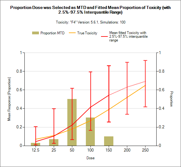
It is common in CRM for the doses to be unequally spaced, if plotted using the dose strength this can lead to very closely spaced results and very narrow results columns. To work around this problem, each graph now includes a “Space doses evenly” option. Here is the same graph, spaced normally and with even spacing:

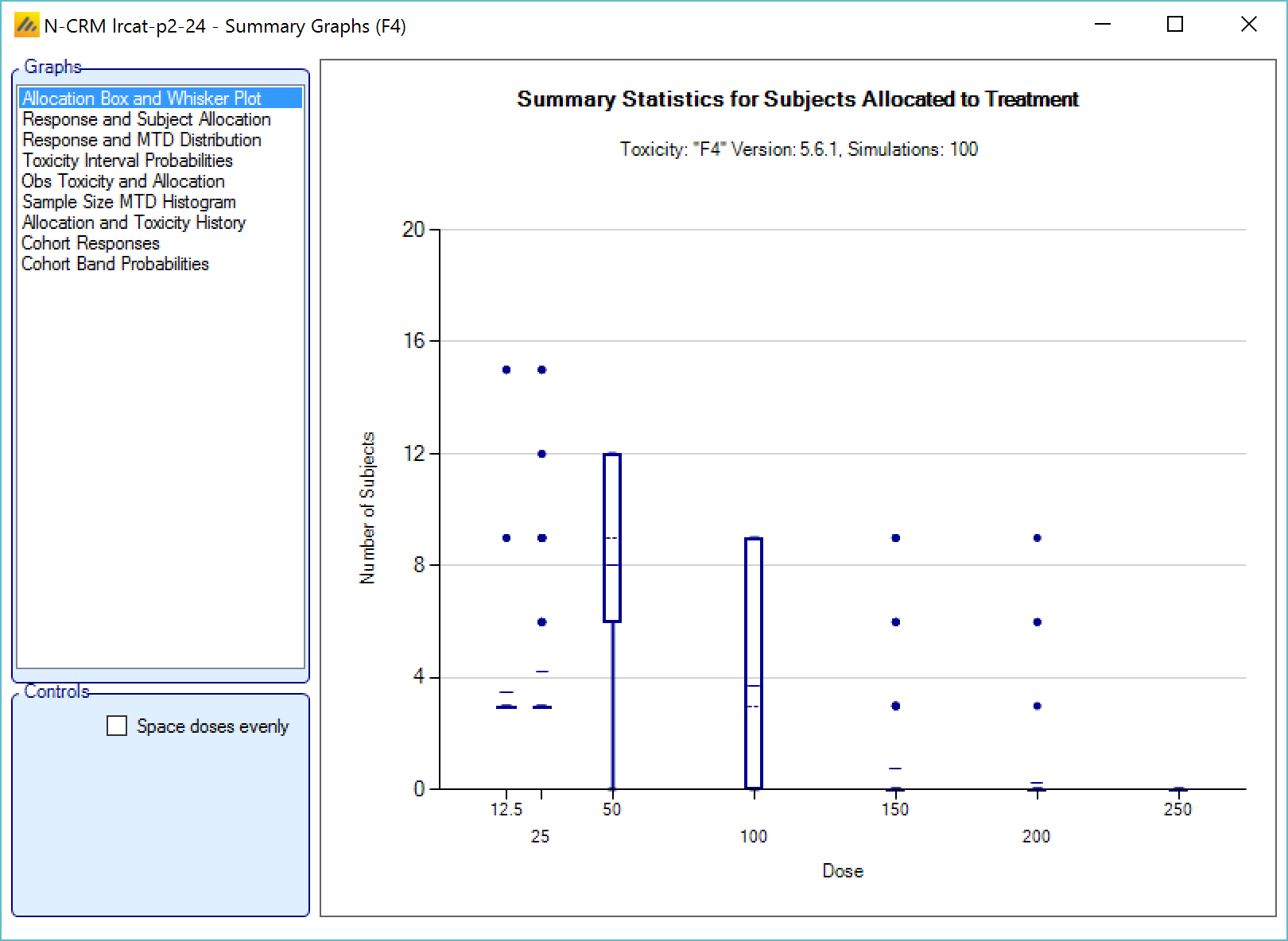
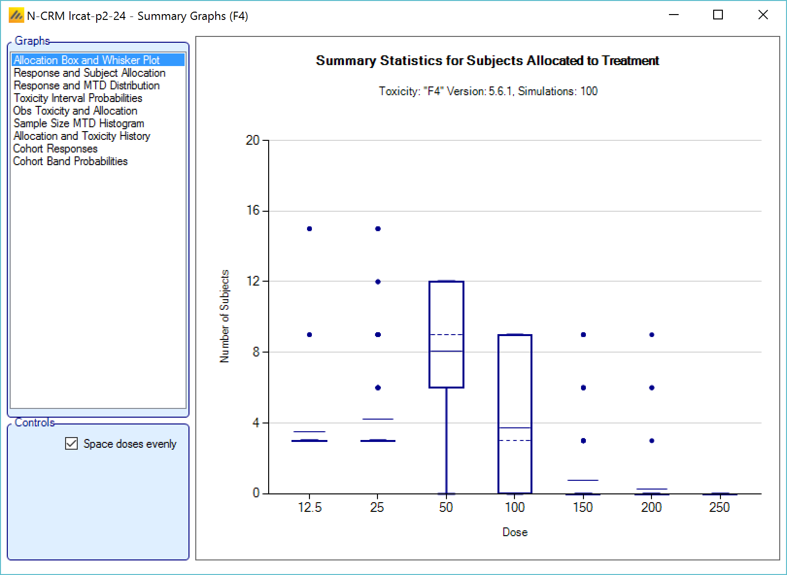
Allocation Box and Whisker Plot

This graph displays a box and whisker plot of the number of subjects allocated to each dose over the simulations. These plots show:

The mean allocation over all simulations at each dose plotted as a solid line.
The median value is plotted as a dashed line.
The 25-75th quantile range is plotted as the “box” portion of each point.
The “whiskers” extend to the largest and smallest values within 1 ½ times the interquartile range from either end of the box.
Points outside the whisker range are considered outliers, and are plotted as small blue dots. Note that it may be difficult to see all of these symbols if they are plotted at the same value.

If 2 groups are simulated, there are two versions of the graph showing the distributions of allocation for each group separately.

Response and Subject Allocation

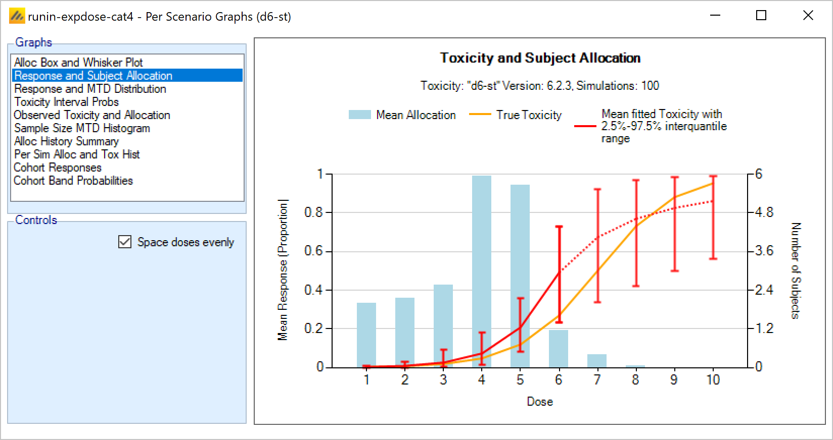
This plot shows the mean subject allocation to each dose as a blue bar, along with lines showing the mean estimated toxicity and the simulated ‘true’ toxicity. The ‘error’ bars on the mean estimated toxicity are the 95% interval of the mean estimates across the simulations.

If 2 groups are simulated, there are two versions of the graph showing the distributions of allocation and the mean fitted toxicity separately.

If efficacy is being simulated, then lines for the mean fitted efficacy and true efficacy are also shown.

Response and MTD Distribution

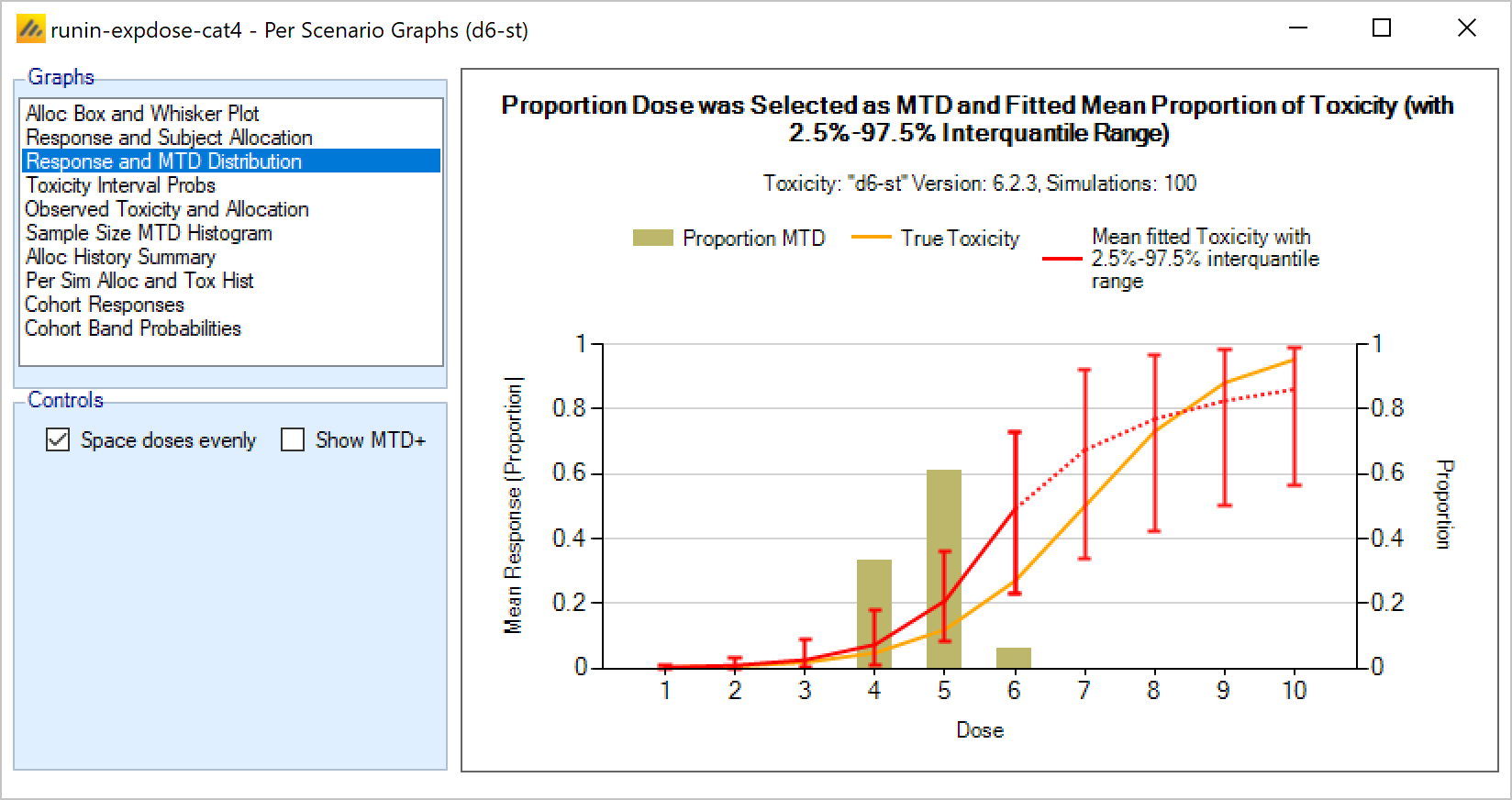
Figure 70: MTD distribution and response graph

This plot shows the proportion of times each dose has been selected as the MTD as a brown bar, along with lines showing the mean estimated toxicity and the simulated ‘true’ toxicity. The ‘error’ bars on the mean estimated toxicity are the 95% interval of the mean estimates across the simulations.

There is an options to display the “MTD+” distribution. This is the proportion of times each dose has been selected as the MTD when a dose below the lowest dose and a dose above the highest dose is included.

If 2 groups are simulated, there are two versions of the graph showing the distributions of allocation for each group separately.

If efficacy is being simulated then there are versions of the graph showing the histograms showing the distribution of selection of MTD, MED, OSD, and TE targets. The plot of the MTD shows the true and mean fitted toxicity, the plot of the MED shows the true and mean fitted efficacy and the plots of the OSD and TE show both the true and mean fitted toxicity and efficacy.

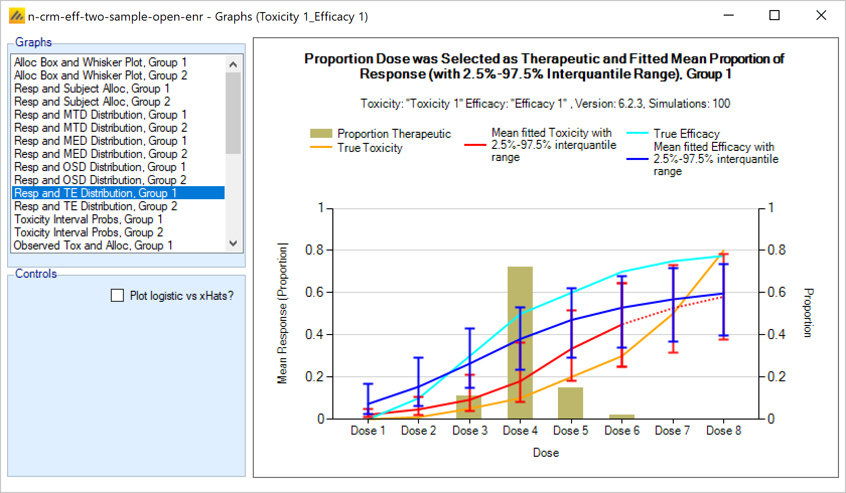
Figure 71: Response and TE Distribution for a group

Toxicity Interval Probabilities

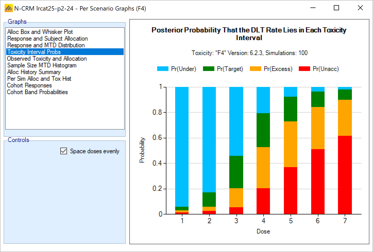
This plot shows the posterior probability for each dose that it’s toxicity rate lies in each of the four toxicity intervals as a stacked bar chart.

Observed Toxicity and Allocation

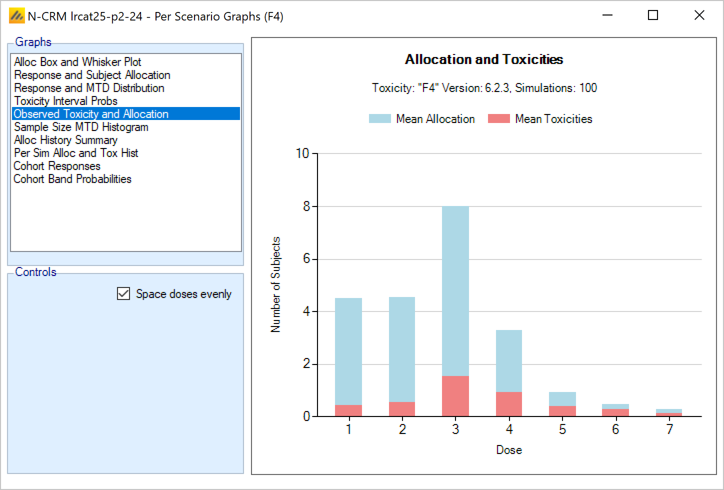
Figure 73: Observed Toxicities and Allocation Histogram

This graph shows the mean allocation to each dose and the mean number of toxicities observed at each dose. The total height of the bar shows the total allocation, and the red section of the bar shows the proportion that experienced toxicity.

Sample Size MTD Histogram

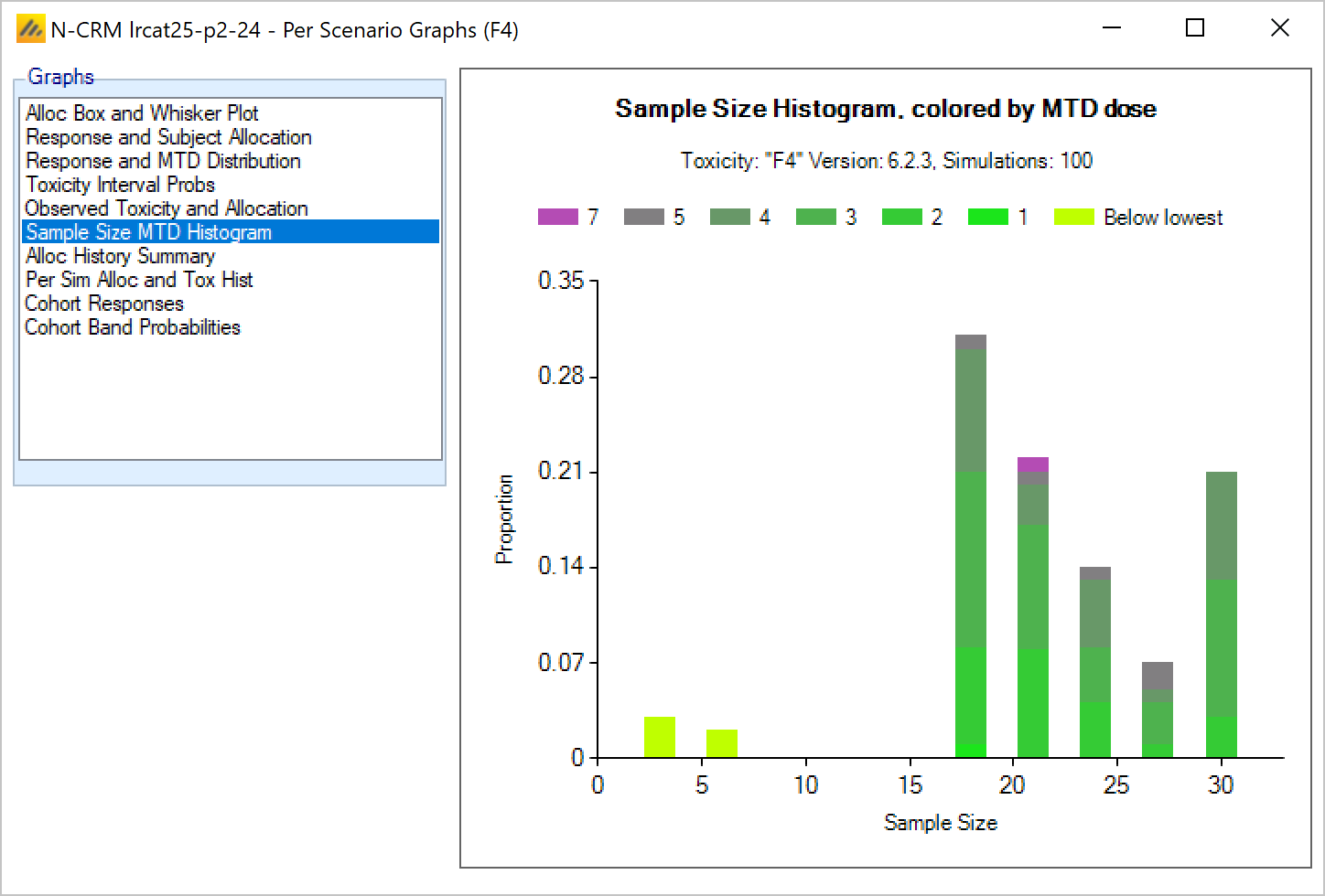
This graph shows the number of times different sample sizes (number of subjects tested) were observed across the simulations. Each bar is shown as a stacked plot with each color indicating the proportion of times a particular dose was selected as the MTD in the simulations that ended with a particular sample size.

Alloc History Summary

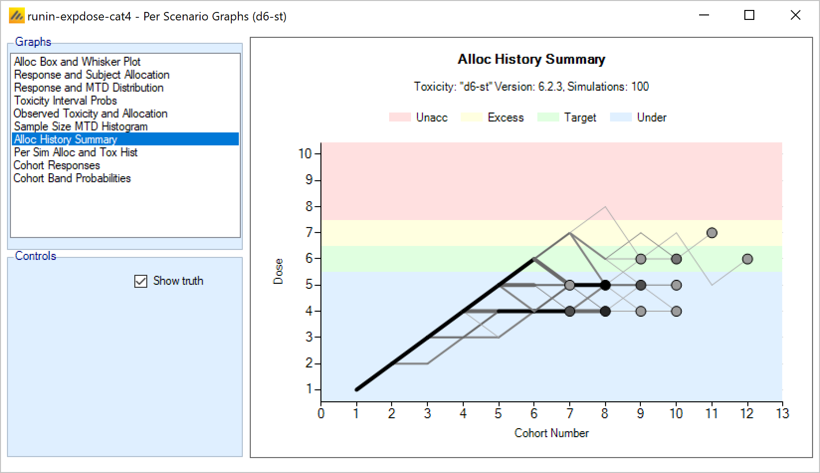
Figure 75: Allocation History Summary Graph

This graph overlays all the allocation histories of those simulations for which “cohorts” files have been output. The lines show the “route” the dose escalation followed and the circles show the dose selected as MTD at the end of the simulation. The lines are heavier and the circles darker the more simulations followed the same route or made the same selection.

There is an option to show “the truth”, which if selected (the default) colors the background according to the simulated toxicity rate of the dose strength on the y-axis. Thus the background has bands of color for “under-dosing”, “target”, “excess” and “unacceptable” toxicity.

This graph allows a quick appraisal of how well the design and priors allow the dose escalation to reach and then stop in the target band.

Per Sim Alloc and Tox History

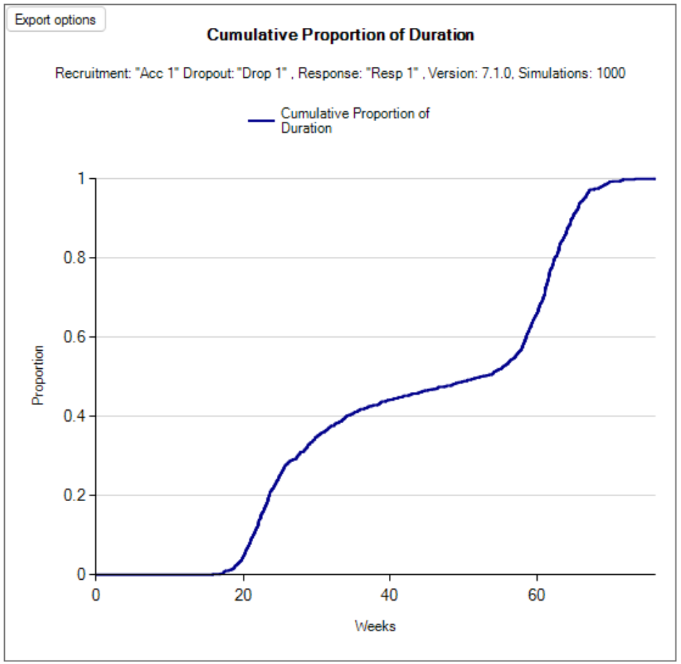
Figure 76: Allocation and toxicity history plot

This graph shows the allocation and toxicity history for an individual simulation. Each dot represents a subject, the dot is colored red if toxicity was observed, grey otherwise. The subjects’ outcomes are displayed left to right in the order in which they were dosed, and at a height corresponding to the dose they were given.

The graph includes a drop down selector box allowing the user to select which simulated trial is displayed. A history can only be displayed for trials for which a ‘cohorts’ file has been written out.

On the left hand side, a black triangle next to the y-axis indicates the highest cleared dose. Green/red triangles show the Model MTD/MED+ and finally the selected MTD/MED.

If the trial uses open enrolment this graph is slightly changed.

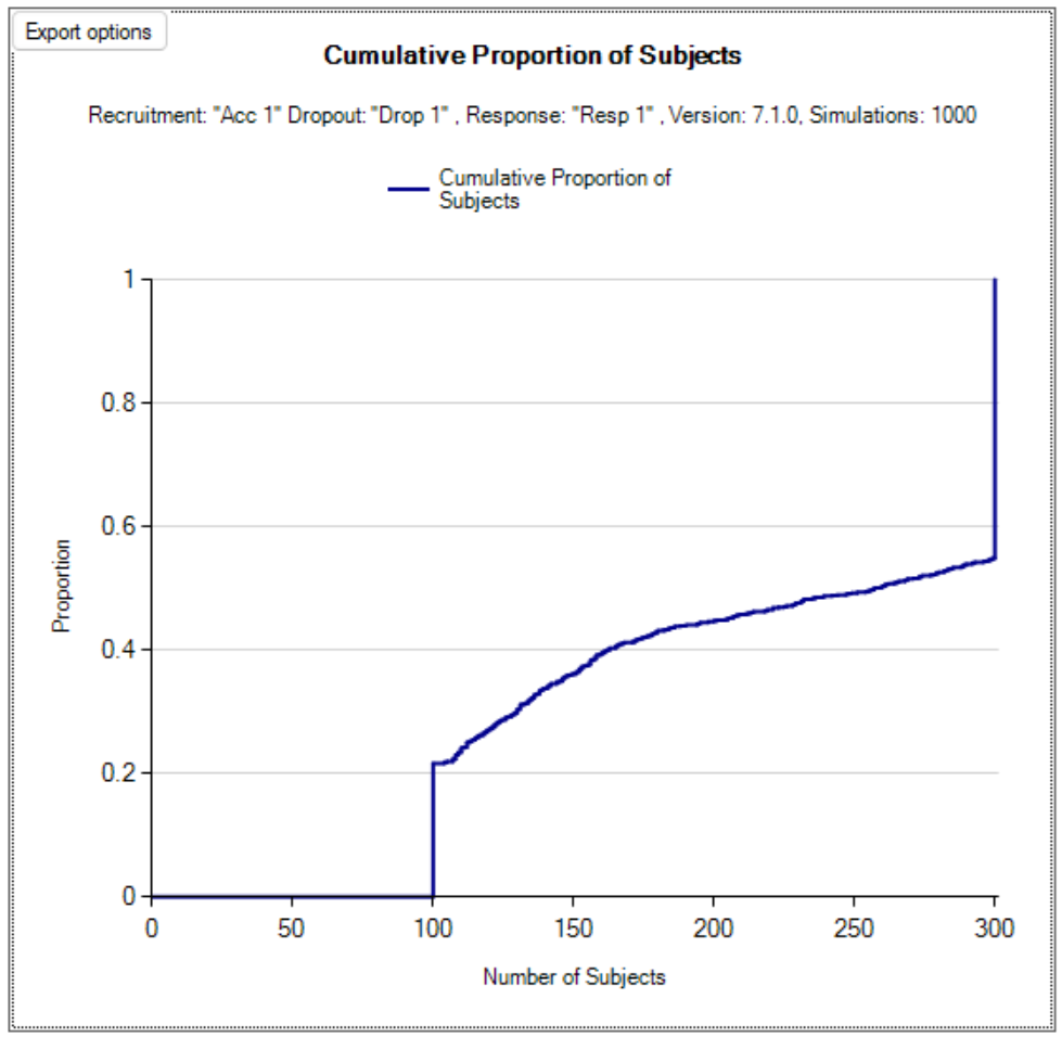
Figure 77: Open Enrolment Allocation and Toxicity History graph

If the trial uses open enrolment then this graph has an “Interim” picker that shows the data available at a specific interim. Subjects whose outcome has not been observed at this interim are shown as grey squares. Subjects who were not included in the trial because there were already the maximum number of subjects treated but who had not attained their final toxicity / non-toxicity status are shown as yellow crosses at the level below the lowest dose. As the interim displayed is increased subjects symbol will change as their endpoint data becomes available.

Cohort Responses

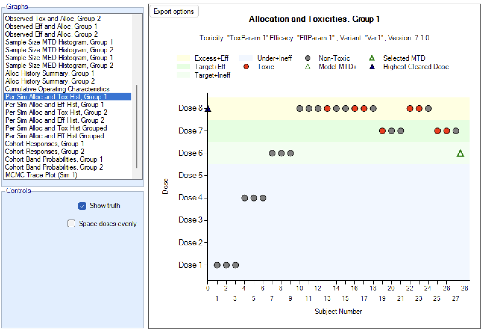
This graph shows the dose allocation and resulting toxicities along with the fitted dose-toxicity model for a single simulated trial after the results have been gathered for a specific cohort of a specific trial.

The graph includes a drop down selector box allowing the user to select which simulated trial is displayed, and a further drop down selector box allowing the user to select at which cohort to display the state of the trial.

These details can only be displayed for trials for which a ‘cohorts’ file has been written out.

It the trial uses open enrolment then subjects whose outcome has not been observed at the time of the interim being displayed are shown as a light grey part of the “allocated subjects” bar.

If trial simulates 2 groups then there are two graphs one for each group.

If the trial simulates efficacy, then the bar shows both toxicities and efficacies using half width bars of different colors.

Green/Red triangles indicate the Model MTD/MED and finally the selected MTD/MED.

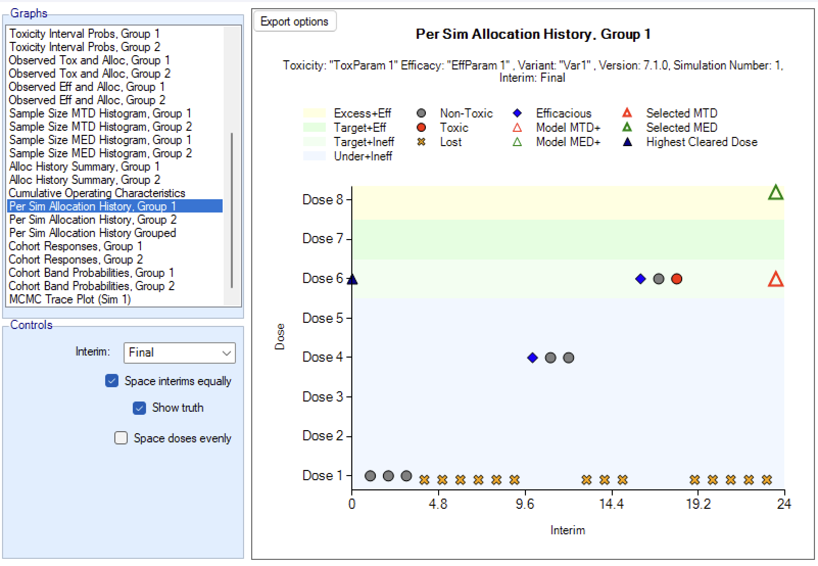
Figure 79: Cohort Responses for one of two groups showing efficacy and toxicity

Cohort Band Probabilities

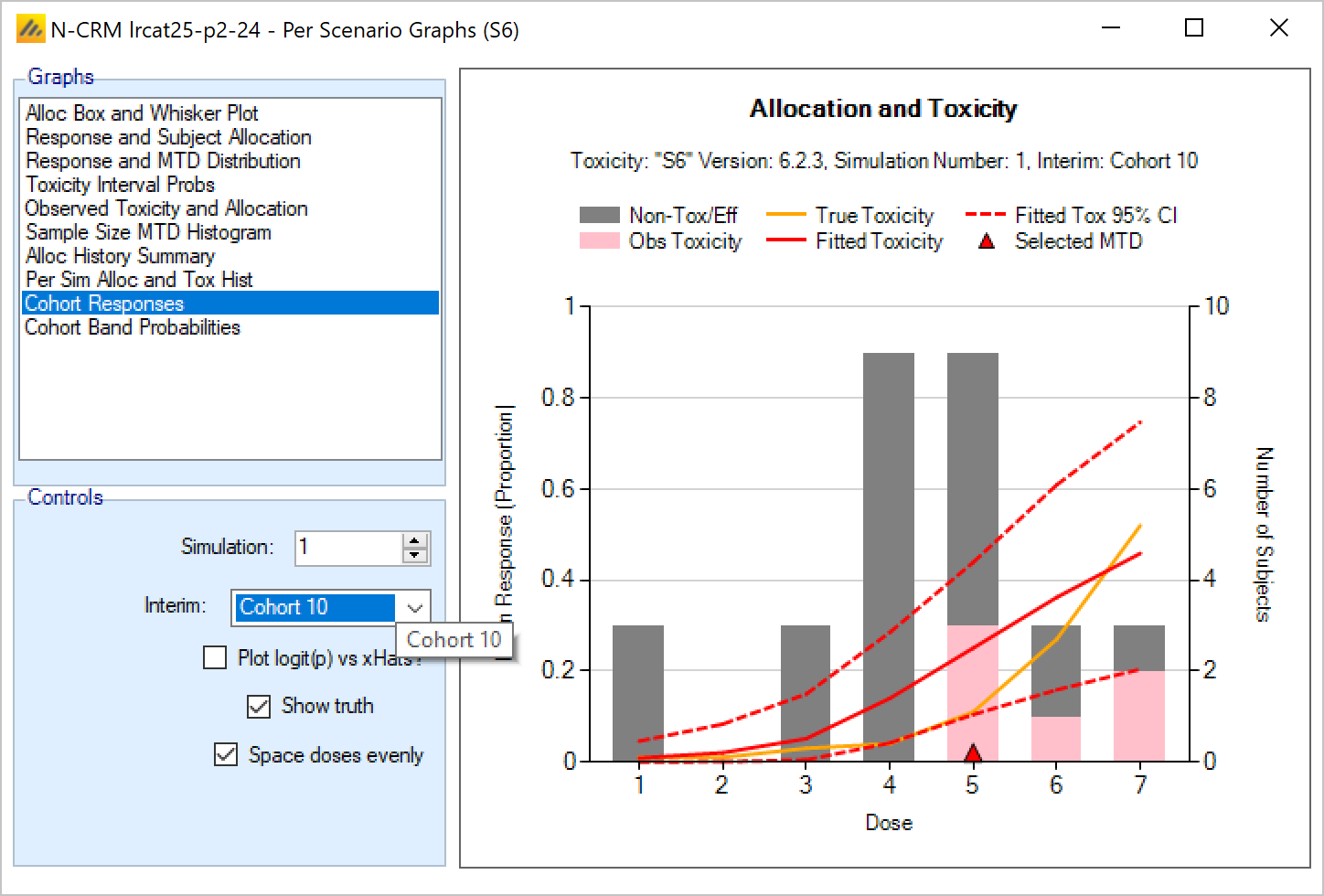
This graph shows the dose allocation and resulting toxicities along with the posterior probabilities that the toxicity rate lies in each of the toxicity bands for each dose, for a single simulated trial after the results have been gathered for a specific cohort of a specific trial.

These details can only be displayed for trials for which a ‘cohorts’ file has been written out.

Green/Red triangles indicate the Model MTD/MED and finally the selected MTD/MED.

MTD Change on Expansion

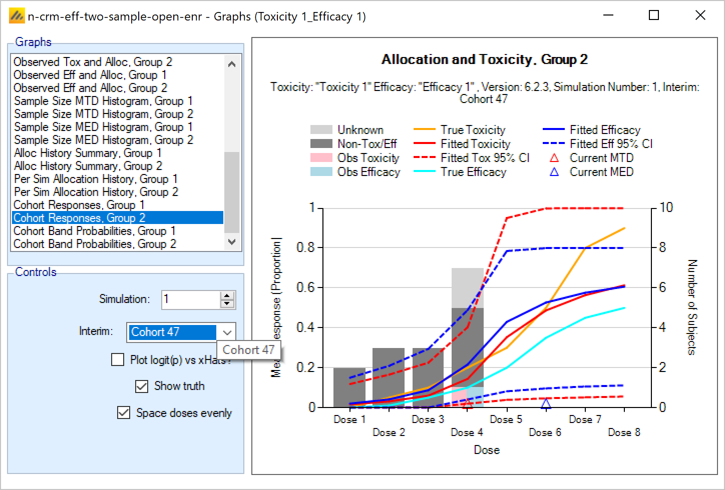
This graph plots the dose selected as MTD before the results of the expansion cohort are available, against the dose selected as MTD after the expansion cohort results are available. Each simulation result is plotted as a ‘dot’, and the graph is divided up into a grid and dots located in the correct cell in the grid and then arranged within the cell depending on how many results fall into the cell. This allows the relative number of results in each cell to be appraised quickly by eye.

This graph allows the trial designer to see the degree of risk that the determination of the MTD will change as a result of the expansion cohort and whether the risk is predominantly that the determination will increase or decrease.

Across Scenario Graphs

To enable swift visualization and comparison of the simulation results across the different scenarios and variants, FACTS has a number of pre-defined graph trellis plots that it can display.

To view these graphs, click on the ‘View Graph’ button and select “Show Across Scenario Graphs”.

As with the per scenario graphs, the display supports copying just the graph to the clipboard, to facilitate pasting them into documents and presentations. Right clicking on a graph brings up a short menu that allows the image of the graph to be copied to the clipboard or saved in ‘png’ format to a file.

The trellis plots all include a “Select Scenarios/Variants…” button that displays a control that allows the variants and scenarios included in the trellis to be filtered:

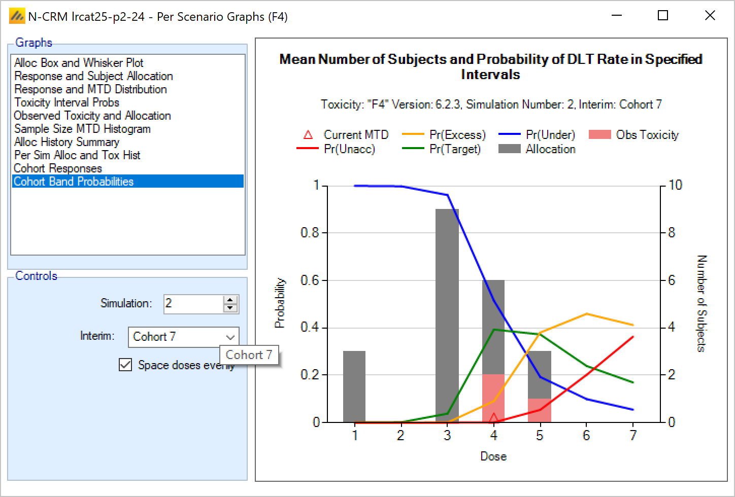
Selected MTD graph

The Selected MTD “Across Scenarios” graph shows for each scenario and each variant a histogram of the proportion of times each dose was selected as the MTD at the end of the simulations in that scenario. The bars are colored to reflect the toxicity band that the “true” toxicity rate of the dose falls into in that scenario.

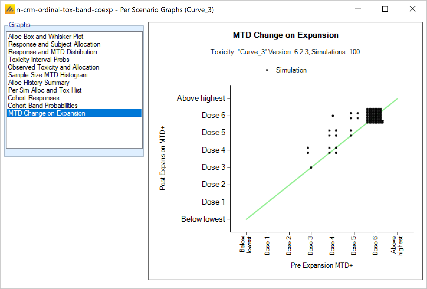
Toxicity Interval Probabilities graph

The Toxicity Interval Probabilities “Across Scenarios” graph shows for each scenario and each variant a stacked bar chart of the posterior probability that the toxicity rate at each dose falls into one of the user defined 4 toxicity bands.

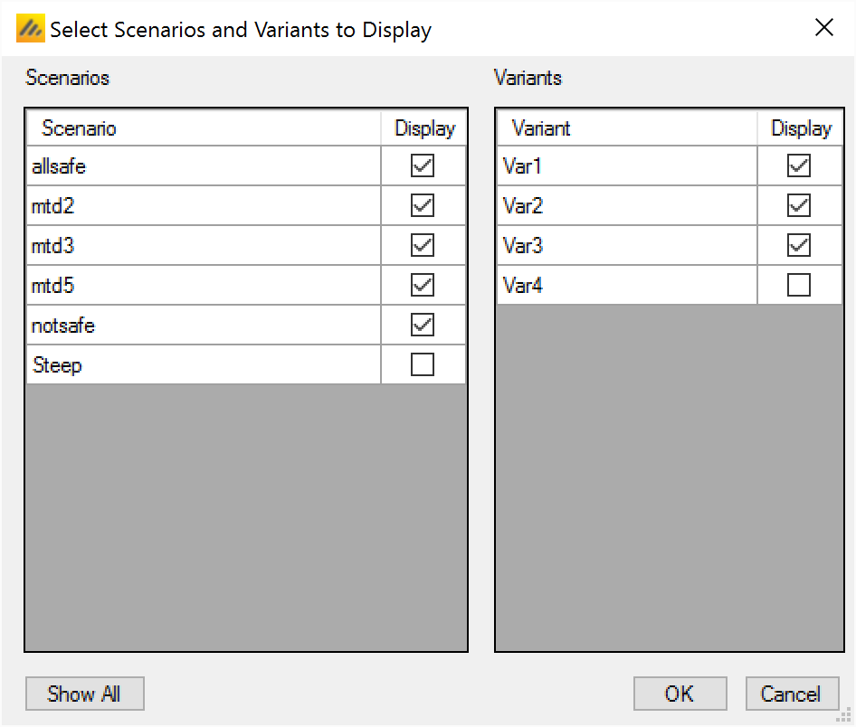
Fitted Toxicity

The Fitted Toxicity “Across Scenarios” graph shows for each scenario and each variant, the mean fitted toxicity and the 95-percentile spread of the fitted toxicities across the simulations.

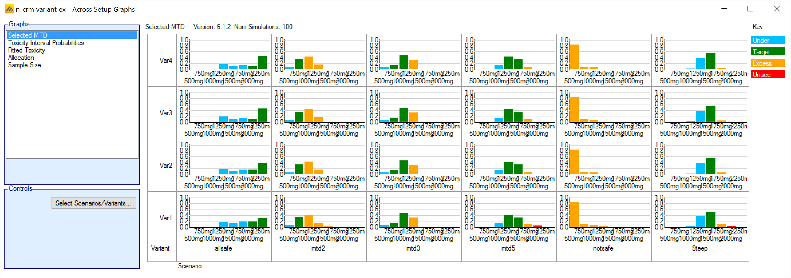
Allocation

The Allocation “Across Scenarios” graph shows for each scenario and each variant, a box plot of the spread of the number of subjects allocated to each dose across the simulations. As N-CRM may only be allocating a small number of cohorts the number of subjects allocated to each dose is often not a smooth distribution, but somewhat discontinuous.

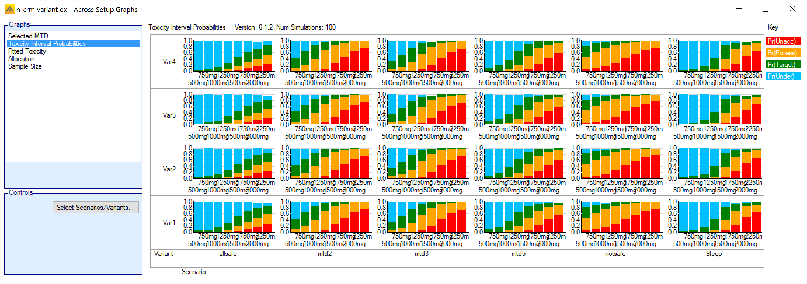
Sample Size

The Sample Size “Across Scenarios” graph is the only “Across Scenario” graph that is not a trellis plot. It is a single graph with a line plotted per scenario of the mean sample size at each maximum sample size.

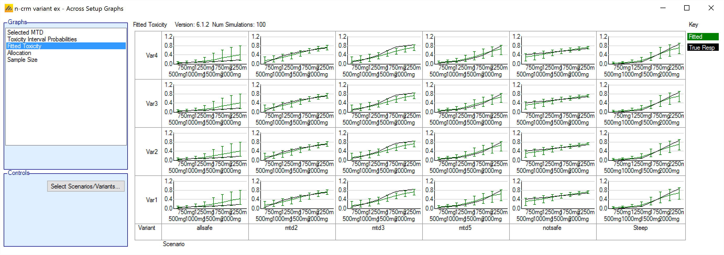
Using the N-CRM Model to analyze data

The N-CRM design engine has built-in GUI support for using the design engine to execute the trial. Using the design engine to analyze a dataset and report the recommended action for the next cohort.

In order to run an N-CRM trial using FACTS the trial design needs to be entered first. The selected design is then opened and converted to running a trial. To do this, open FACTS with the design to be used to run the trial and open the analysis tab:

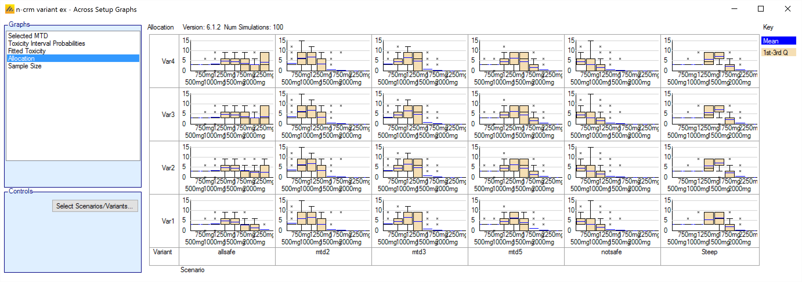
Figure 88: Recommender Tab, before converting to a trial

Clicking on the “Use Design to Analyze Data” button, will create an empty “subject.csv” file in the main simulation results directory and a sub-directory there for running the design recommender and saving the outputs. It is not possible to change these locations once created, so use SaveAs first if you wish these to be in a new location.

Alternatively, clicking on the “Import Data to Analyze” launches a file browser, allowing the user to select a ‘.csv’ file to load as the data to analyze. This is a shortcut for first clicking on the “Use Design to Analyze Data” button, and then clicking on the “Select File to Create New Analysis” button on the subject data tab.

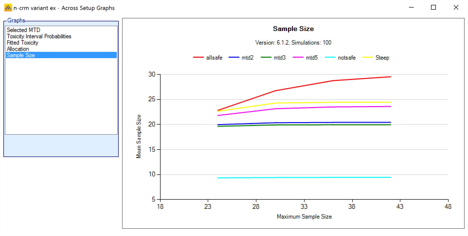
Figure 89: Recommender Tab, after enabling analysis

After enabling data analysis, the analysis screen is shown with no data loaded. By clicking on the “Subject Data” tab the user is now able to enter data values directly, or to load a ‘.csv’ file already containing data:

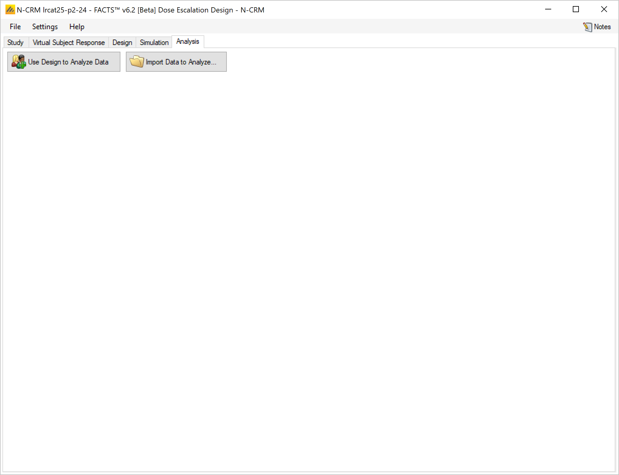
Entering the data directly

The data can be entered directly in the data grid – each row containing the date for a single subject.

The format of the grid is the same as though viewing the “subject.csv” file in a spreadsheet.

For historical reasons the data file format contains 5 columns that are now unused but have been retained. Thus the columns are:

First column is the subject ID. This column can be left blank, FACTS does not used the value, it is there to allow the data to be cross-referenced to an external data source. If not required there is no harm simply entering ‘1’ on each row.
The next 5 columns are unused and can be left blank. Do not enter text containing comma’s in these fields, these will be read as column separators if the data is saved and read back in.
Cohort number, this should be an integer indicating which cohort the subject belonged to (and hence the order in which they entered the trial). This data is sometimes used when determining what doses the allocation rules permit to be used. The FACTS GUI now checks to ensure that this value has been entered.
Dose Strength, if explicit doses are being used this value must match the dose strength of one of the doses defined on the ‘Treatment Arms’ tab – as the dose escalation rules are defined in terms of “number of doses”. If doses have been defined using ‘finely spaced doses’ then this column can contain any value as dose escalation rules defined using “dose strength”. The value entered will be used as the strength of the dose the subject was administered.

Apart from the requirement that the dose strength corresponds to one of the planned doses if the design uses explicit doses, there is no need for the data entered to represent a dose escalation permitted by the design. The team can have been more or less cautious, and there can be more or less data, than originally planned.
Toxicity – if a binary endpoint is being used this must be 0 (not-toxicity) or 1 (toxicity), if Ordinal toxicity is being used then this must be 1, 2, 3 or 4; where 1 is now no toxicity, 2 mild toxicity, 3 toxicity, and 4 severe toxicity.
Efficacy – this must be 0 (no efficacy) or 1 (efficacy), even if efficacy is not being modelled in the design. If it is not being modelled then whether the value is 0 or 1 is immaterial.

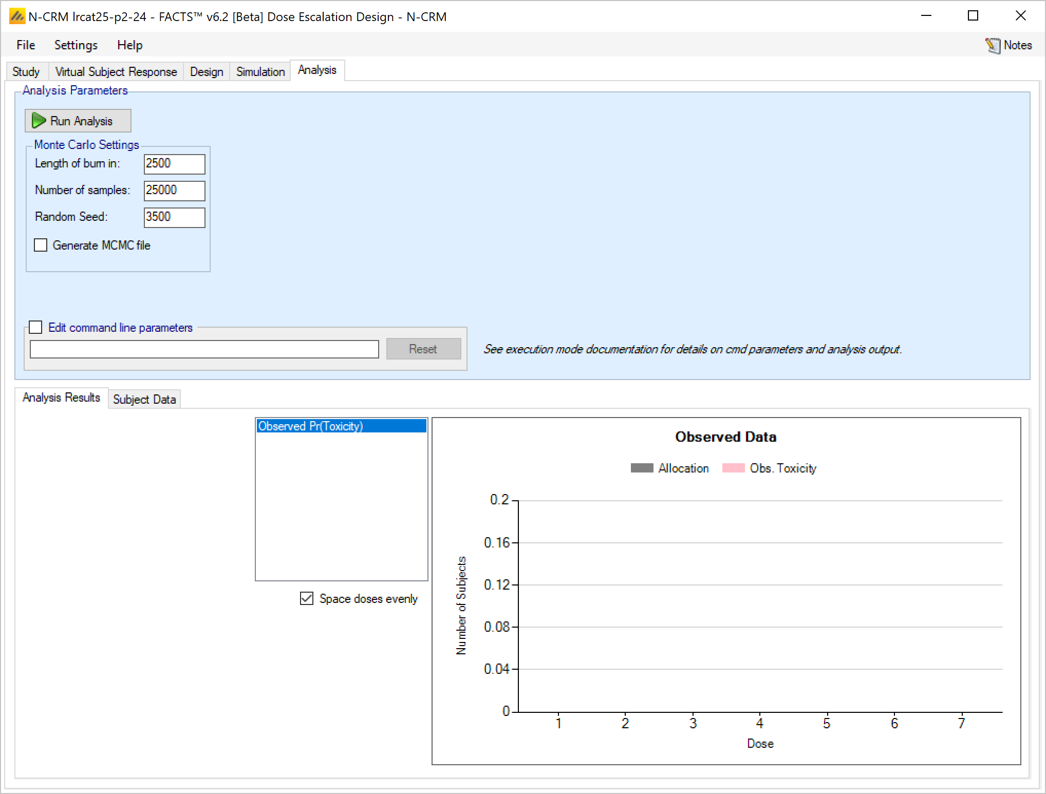
If the data entered and then ‘Run Analysis’ clicked, the data is saved to a file called ‘subject.csv’ and the analysis results saved to a folder called ‘Analysis’ within the “_results” folder of the design.

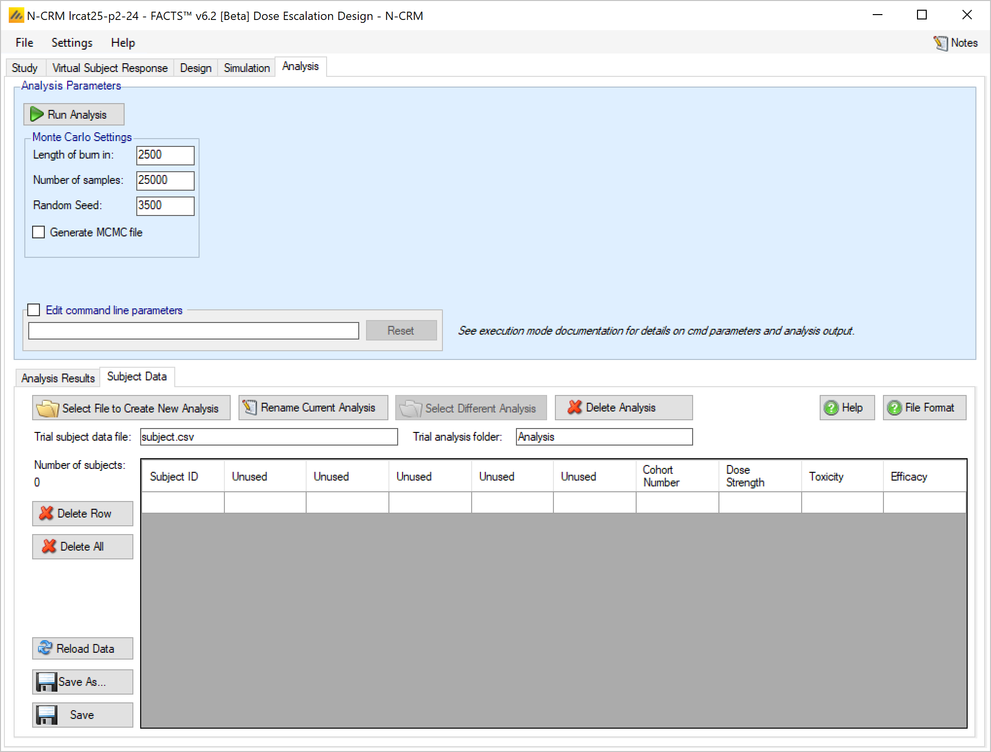
The ‘Save As’ button can be used to save the file with a different name, but it will still be saved within the _Results folder.

A specific results folder is also created, called ‘Analysis_’.

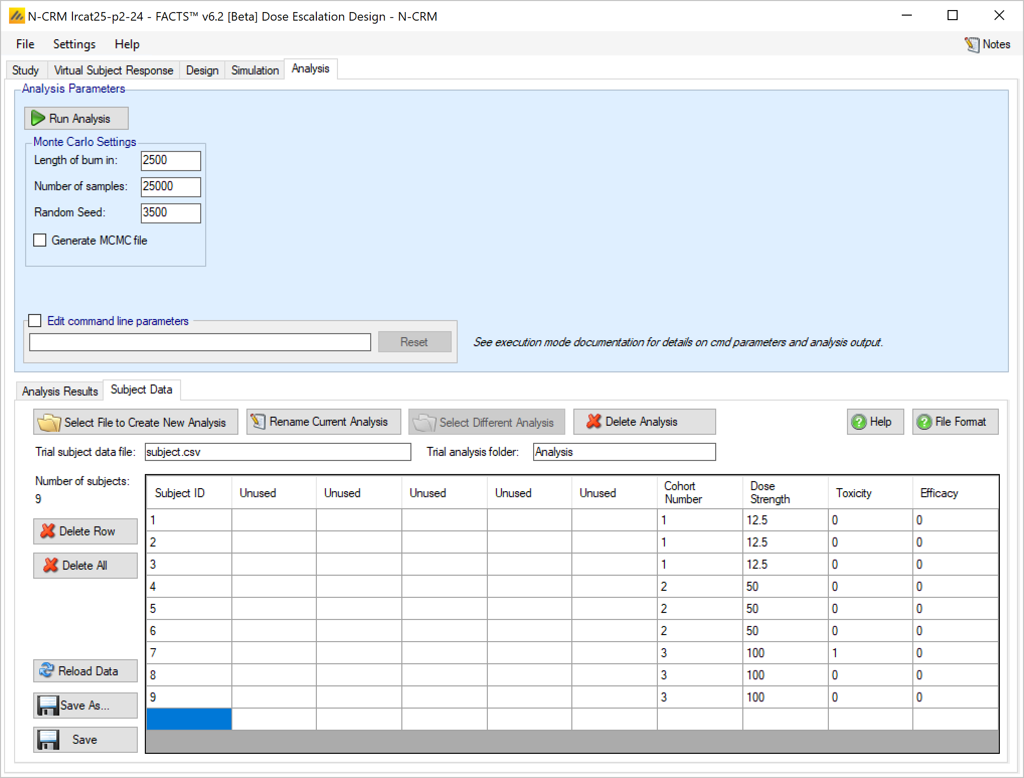
Loading Data From a File

As well as entering the data via FACTS its possible to load the data from a ‘subject.csv’ file. These can be cerated within FACTS or outside of FACTS and once created can be edited FACTS or outside of FACTS.

We have tried to make it particularly easy to enter, modify and analyze data in N-CRM because this is a useful way to explore the properties of the design in addition to simulation.

The subject.csv file format

The file is a simple ascii file with the different data items separated by commas. Any line starting with ‘#’’ is ignored, here we use that to include a header row. The data may also include spaces to aid readability (but not, currently, tabs). Each line defines the dose given to a single subject and that subject’s response.

For historic reasons the CRM subject.csv file format includes fields for patient identification data, however the FACTS design engine does not use this data, but does require that the columns contain data of the expected format. This is the first 6 columns: patient ID, Patient Initials, Year, Month, Day, Time & Cohort. The simplest thing to do is enter simple default values as shown below.

#Patient ID, Patient Initials, Year, Month, Day, Time, Cohort, Dose, Toxicity, Efficacy
1, , , , , , 1, 12.5, 0, 0
In FACTS only the last four columns are ever significant: Cohort, Dose, Toxicity and Efficacy. “Dose” needs to contain the dose level (not the dose index)) of the dose given to the subject, For example if the dose levels were specified as 12.5, 25, 50, 100, 150, 200 and 250 so this column should contain one of these values.

If the toxicity endpoint is dichotomous then “Toxicity” needs to contain either a ‘1’ (to indicate toxicity observed) or a ‘0’ (for no toxicity). If its ordinal, then it needs to contain a ‘1’, ‘2’, ‘3’ or ‘4’ corresponding to the observed level of toxicity for that subject, where ‘1’ is now “no toxicity’ and ‘3’ is the ‘target toxicity’, ‘2’ is ‘mild toxicity’ and ‘4’ is ‘severe toxicity’.

A value in the final “Efficacy” column is also required whether or not efficacy is being modelled in the design. The column should contain either a ‘1’ (to indicate efficacy observed) or a ‘0’ (for no efficacy).

Thus if the first cohort had been allocated the lowest dose ’12.5’ and no subjects experienced toxicity (‘0’), the subjects.csv file looks like this:

#Patient ID, Patient Initials, Year, Month, Day, Time, Cohort, Dose, Tox, Efficacy
1, , , , , , 1, 12.5, 0, 0
1, , , , , , 1, 12.5, 0, 0
1, , , , , , 1, 12.5, 0, 0

Data file management on the Analysis tab

From FACTS 6.2 onwards FACTS now supports multiple subject data files and analysis folders.

Buttons that allow the subject data file to be changed:

’Select File to Create New Analysis: launches a file browser that allows the user to select a new “.csv” file from any location. The selected file is copied to the “_Results” folder (retaining its current name) and made the current subject data file.
‘Rename Current Analysis’ allows the name of the current subject data file to be changed.
‘Select Difference Analysis’ allows a different subject data file that is in the “_Results” folder to be made the current subject data file.
‘Delete Analysis’ allows any of the subject data files that are in the “_Results” folder to be deleted.

The name of the current subject data file and the name of the corresponding analysis folder are shown below the subject data file buttons.

There are five buttons that allow the currently loaded subject data file to be modified:

‘Delete Row’ deletes the currently selected row in the data grid. The data in the current subject file is not updated unless the current data is saved.
‘Delete All’ clears all the data in the data grid. The data in the current subject file is not updated unless the current data is saved.
‘Reload data’ replaces the data in the data grid with the data that is still in the current subject data file.
‘Save As’ saves the current data in the data grid to a new subject data file in the “_Results” folder, and makes that the current subject data file.
“Save” saves the current data in the data grid to the current subject data file.

Running an analysis performs a ‘Save’ before running the analysis.

Running an Analysis

Once data has been loaded or entered, the user can click the ‘Run Analysis’ button.

Once the analysis has run, FACTS displays the recommendation, and a graph showing the data the fitted toxicity.

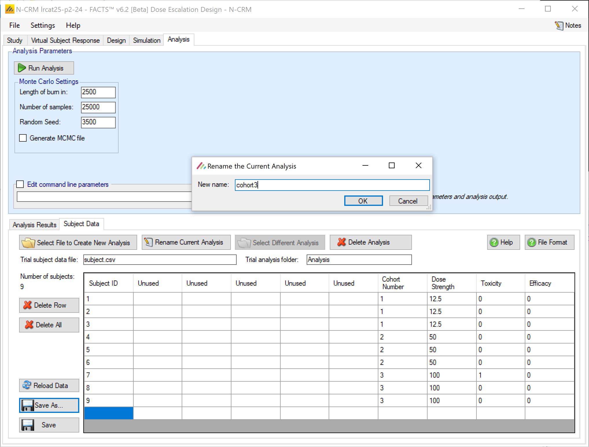
Figure 95: Analysis tab - analysis results

The available analysis parameters are

MCMC Burn-in: how many of the initial MCMC samples are discarded before accumulating samples to estimate the posterior distributions of the values of interest.
Number of samples: the number of MCMC samples to take in-order to estimate the posterior distributions of the values of interest.
Random Seed: the seed to be used initialize the random number sequence, with the same design data and random seed FACTS will return the same results.
Edit command parameters. This allows the command line string to the design engine to modified, this is an advanced option. The command line options are described in the “FACTS DE User Guide for Trial Execution”.

Analysis Graphs

Three graphs are available, the first shows the subject allocation, observed toxicities and resulting fitted curve:

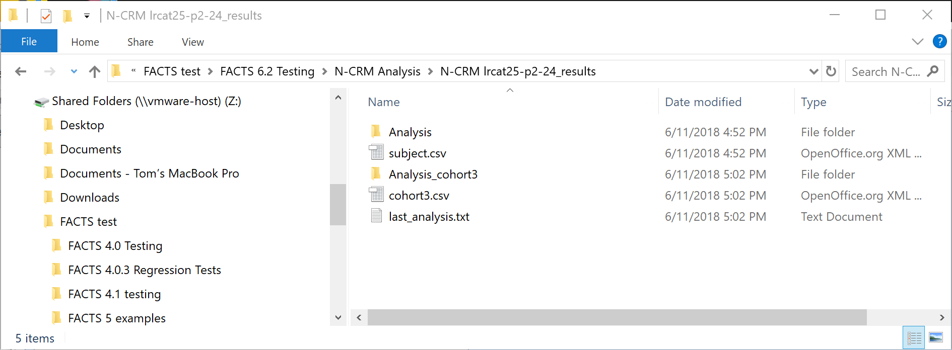
The second shows the posterior probabilities for each dose that its toxicity rate falls in each of the 4 toxicity bands:

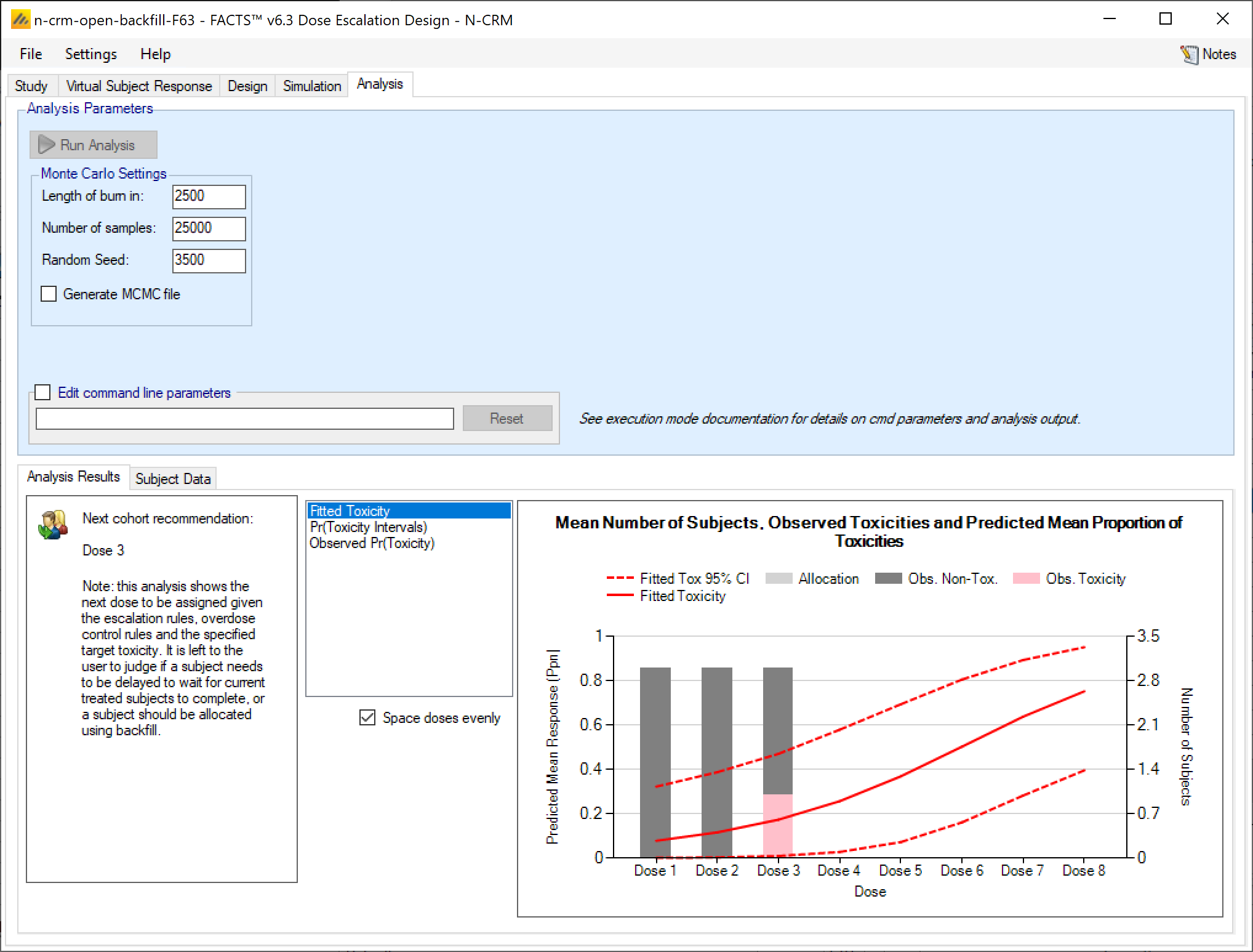
The third simply shows the observed data:

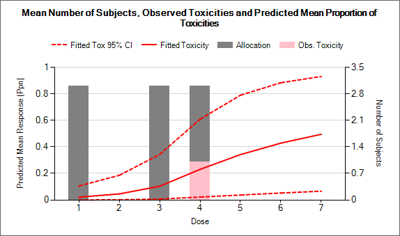
A fourth graph is available if “Generate MCMC file” is checked before running the analysis, we can now view MCMC trace plots of the fitted parameters such as Alpha and Beta:

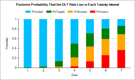
Output Files

FACTS stores the results of simulations as ‘.csv’ files under a Results folder. For each row in the simulations table, there is a folder named by the toxicity response profile, which contains the corresponding ‘.csv’ files.

These files can be opened using Microsoft Excel, but versions of Excel before 2007 are restricted to 256 columns, which is too few to view some files in their entirety. OpenOffice Calc will show all the columns (and will allow you to open two files that have the same name at the same time!). Because Excel takes out a file lock on any file it has open, while a file is open in Excel it cannot be deleted or modified by another application. The most common cause for an error to be reported when simulating trials in FACTS is because the user has one of the previous results files is still open in Excel.

There are several types of file:

Summary.csv contains a single row of data that holds data summarized across the simulations. This is the source of most of the values in the simulations table.

Simulations.csv contains one row per simulation describing the final state of each simulation for every trial simulated.

CohortsNNN.csv contains one row for each cohort during a simulation where NNN is the number of the simulation. By default this file is written only for the first 100 simulations, but this can be changed via the advanced button on the simulation tab. The values in the last row of the cohorts file will be the same as the final values for that simulation in the simulations file.

Contents of summary.csv

The columns in summary.csv are common across all the FACST Dose Finding design engines.

Some columns are only output if certain options are being used:

Efficacy Only These columns are output only if an efficacy endpoint is simulated as well as the toxicity endpoint.

Open Enrolment Only These columns are output only if open enrolment is being simulated rather than cohort enrolment.

Cohort Expansion Only These columns are output only of an expansion cohort is being simulated.

MTD only These columns are output only if the target dose for the toxicity endpoint is a single MTD, rather than the dose most likely to have a toxicity rate in the target toxicity band.

If 2 groups are being simulated, then there are two separate summary files. The first summary file “summary.csv” contains the results for the first group, the second summary file “summary2.csv” contains the result for the second group.

Column Title	Number of columns	Description
Number of Sims	1	The number of simulations that were run to produce the displayed results.
Random Number Seed	1	The random number seed used to simulate the scenario.
Mean num subjects	1	This is the mean (over the simulations) of the number of subjects recruited in this scenario (including any single patient run-in, but excluding any expansion cohort..
Ppn Tox	1	This is the average proportion of the subjects recruited that experienced a toxicity in this scenario.
Ppn Eff	1 – Efficacy only	This is the average proportion of the subjects recruited that experienced a efficacy in this scenario.
SD Ppn Tox	1	This is the standard deviation of the proportion of toxicity across the simulations.
SD Ppn Eff	1 – Efficacy only	This is the standard deviation of the proportion of efficacy across the simulations.
True Mean Tox	1	This is the average true probability of toxicity over the simulations. The ‘true probability of toxicity’ in a simulated trial is the average of the probabilities of toxicity all the subjects are exposed to, given the toxicity response profile that we are simulating from.
True Mean Eff	1 – Efficacy only	This is the average true probability of efficacy over the simulations. The ‘true probability of efficacy’ in a simulated trial is the average of the probabilities of efficacy all the subjects are exposed to, given the efficacy response profile that we are simulating from.
Mean Beta Tox	1	This is the mean (over the simulations) of the mean of the posterior distribution of the estimate of the Beta parameter of the toxicity logistic model.
s.d.Beta Tox	1	This is the mean (over the simulations) of the standard deviation of the posterior distribution of the estimate of the Beta parameter of the toxicity logistic model.
Mean Alpha 3 Tox	1	This is the mean (over the simulations) of the mean of the posterior distribution of the estimate of the Alpha 3 parameter of the toxicity logistic model.
s.d.Alpha 3 Tox3	1	This is the mean (over the simulations) of the standard deviation of the posterior distribution of the estimate of the Alpha 3 parameter of the toxicity logistic model.
Mean Beta Eff	1 – Efficacy only	This is the mean (over the simulations) of the mean of the posterior distribution of the estimate of the Beta parameter of the efficacy logistic model.
s.d.Beta Eff	1 – Efficacy only	This is the mean (over the simulations) of the standard deviation of the posterior distribution of the estimate of the Beta parameter of the efficacy logistic model.
Mean Alpha 3 Eff	1 – Efficacy only	This is the mean (over the simulations) of the mean of the posterior distribution of the estimate of the Alpha parameter of the efficacy logistic model.
s.d.Alpha 3 Eff	1 – Efficacy only	This is the mean (over the simulations) of the standard deviation of the posterior distribution of the estimate of the Alpha parameter of the efficacy logistic model.
MTD Selection <dose index>	One per dose	For each dose, this is proportion of the simulations where it was selected as the MTD at the end of the study, as defined by the Selected MTD simulation results column. Index starts at 0 if a control arm is included.
MED Selection <dose index>	One per dose – Efficacy only	For each dose, this is proportion of the simulations where it was selected as the MED at the end of the study, as defined by the Selected MED simulation results column. Index starts at 0 if a control arm is included.
OSD Selection <dose index>	One per dose	Unused [it contains values that are copies of the MTD selection. OSD = Optimum Safe Dose, it differs from the MTD only if there is an efficacy endpoint to take into account too]
Mean num Ph1	1 – Efficacy only	This is the mean (over the simulations) of the number of subjects dosed during the first phase of the trial that targets the MTD.
Mean Fitted Toxicity <dose index>	One per dose	This is the mean (over the simulations) of the mean estimate of toxicity from the fitted toxicity response model for each dose.
SD Fitted Toxicity <dose index>	One per dose	This is the standard deviation of the mean estimates across the simulations for each dose. Note it is not based on the standard deviation estimated in the simulations, it is the SD observed across the simulation results.
Mean Fitted Efficacy <dose index>	One per dose – Efficacy only	This is the mean (over the simulations) of the mean estimate of toxicity from the fitted toxicity response model for each dose.
SD Fitted Efficacy <dose index>	One per dose -	This is the standard deviation of the mean estimates across the simulations for each dose. Note it is not based on the standard deviation estimated in the simulations, it is the SD observed across the simulation results.
Mean Subj per dose<dose index>	One per dose	This is the mean (over the simulations) of the number of subjects assigned to each dose.
SD Subj per dose <dose index>	One per dose	This is the standard deviation of the number of subjects assigned to each dose across the simulations.
Mean Tox per dose <dose index>	One per dose	This is the mean (over the simulations) of the number of toxicities observed at each dose.
SD Tox per dose <dose index>	One per dose	This is the standard deviation of the number of toxicities observed at each dose across the simulations.
Mean Eff per dose <dose index>	One per dose -Efficacy only	This is the mean (over the simulations) of the number of efficacies observed at each dose.
SD Eff per dose <dose index>	One per dose – Efficacy only	This is the standard deviation of the number of efficacies observed at each dose across the simulations.
Mean Known per dose <dose index>	One per dose	The number of known patient outcomes for a dose. In N-CRM there is no simulation of drop-outs so this will always be the same as “Mean subj per dose”
SD Known per dose <dose index>	One per dose	This is the standard deviation of the number of known patient outcomes for each dose across the simulations. In N-CRM there is no simulation of drop-outs so this will always be the same as “SD subj per dose”
Num subj 80%ile	1	This is the eightieth percentile across the simulations of the number of subjects recruited into the trial.
Tox Stopping 1	1	The number of times that toxicity stopping rule 1 was true at the end of the simulation. This is the rule that the trial should stop when the specified minimum number of cohorts has been allocated to the dose currently selected as the MTD.
Tox Stopping 2	1	The number of times that toxicity stopping rule 2 was true at the end of the simulation. This is the rule that the trial should stop when no more than the specified number of doses within the credible interval for the target toxicity.
Tox Stopping 3	1	The number of times that toxicity stopping rule 3 was true at the end of the simulation. This is the rule that the trial should stop when a dose achieves the minimum posterior probability of having a toxicity rate within the target band/of being MTD.
Tox Stopping 4	1	The number of times that toxicity stopping rule 4 was true at the end of the simulation. This is the rule that the trial should stop if testing another cohort and observing no toxicities does not change the dose selected as the MTD.
Tox stopping 5	1	Number of times that the maximum cohorts /subjects on MTD was met at the end of a simulation.
Eff Stopping 1	1 – Efficacy only	Number of times the minimum cohorts / subjects on MED was rule was met at the end of a simulation.
Eff Stopping 2	1 – Efficacy only	Number of times the range of dose strengths within the credible interval of the estimate of the dose strength of the MED is less than the specified number.
Eff Stopping 3	1 – Efficacy only	Number of times that the probability that the dose was MED the stopping rule threshold was met at the end of a simulation.
Mean Tox CI	1 – MTD target only	The mean number of doses in the MTD CI
SD Tox CI	1 – MTD target only	The SD of the number of doses in the MTD CI
Mean Eff CI	1 – Efficacy only	The mean number of doses in the MED CI
SD Eff CI	1 – Efficacy only	The SD of the number of doses in the MED CI
Pr(MTD) <dose index>	One per dose – MTD target only	The mean probability of the dose being MTD
Pr(MED)	One per dose – Efficacy only	The mean probability of the dose being the MED
MTD+ <1	1	The number of times the MTD was deemed to be less than the lowest dose
MTD+ <dose index>	One per dose	The number of times each dose was selected as the MTD
MTD+ ><D>	1	The number of times the MTD was deemed to be above the highest dose
MED+ <1	1 – Efficacy only	The number of times the MED was deemed to be less than the lowest dose
MED+ <dose index>	One per dose – Efficacy only	The number of times each dose was selected as the MED
MED+ ><D>	1 – Efficacy only	The number of times the MED was deemed to be above the highest dose
OSD+ <1	1	The same as MTD+ <1, can be ignored
OSD+ <dose index>	One per dose	The same as MTD+ <dose index>, can be ignored
OSD+ ><D>	1	The same as MTD+ > <D>, can be ignored
DE Version	1	This is the version of the N-CRM design engine that simulated these trial results.
GUI Version	1	This is the version of the FACTS GUI that was used to specify the parameters for the trials to be simulated.
Project	1	The name of the project or design
Scenario	1	The name of the scenario within the project or design
Date/Time	1	The date and time the simulations were started
Best <dose index>	One per dose – Efficacy only	The probability that the dose is ‘the best’ – that is it has the highest probability of efficacy without toxicity.
Pr(MTD+) 0	1 – MTD target only	The mean probability that the MTD is below the lowest dose
Pr(MTD+) <D+1>	1 – MTD target only	The mean probability that the MTD is above the highest dose
Pr(MED+) 0	1 – Efficacy only	The mean probability that the MED is below the lowest dose
Pr(MED+) <D+1>	1 –Efficacy only	The mean probability that the MED is above the highest dose
Pr(Under) <dose index>	One per dose	This is the mean (over the simulations) of the posterior probabilities of having a toxicity in the ‘Under-dosing’ toxicity band for each dose.
Pr(Target) <dose index>	One per dose	This is the mean (over the simulations) of the posterior probabilities of having a toxicity in the ‘Acceptable’ toxicity band for each dose.
Pr(Excess) <dose index>	One per dose	This is the mean (over the simulations) of the posterior probabilities of having a toxicity in the ‘Excess’ toxicity band for each dose.
Pr(Unacc) <dose index>	One per dose	This is the mean (over the simulations) of the posterior probabilities of having a toxicity in the ‘Unacceptable’ toxicity band for each dose.
Prior Mean ln(Beta) Tox	1	The value used for the mean value for the prior distribution of log Beta in the toxicity model for all simulations
Prior s.d.(Beta) Tox	1	The value used for the standard deviation of the prior distribution of log Beta in the toxicity model for all simulations
Prior Mean Alpha Tox	1	The value used for mean value for the prior distribution of Alpha in the toxicity model for all the simulations
Prior s.d.Alpha Tox	1	The value used for the standard deviation of the prior distribution of Alpha in the toxicity model for all simulations
Prior Mean Rho Tox	1	The value used for the correlation between Alpha and log Beta in the bivariate Normal prior distribution for Alpha and log Beta in the toxicity model for all simulations
Prior Mean ln(Beta) Eff	1 – Efficacy only	The value used for the mean value for the prior distribution of log Beta in the efficacy model for all simulations
Prior s.d.(Beta) Eff	1 – Efficacy only	The value used for the standard deviation of the prior distribution of log Beta in the efficacy model for all simulations
Prior Mean Alpha Eff	1 – Efficacy only	The value used for mean value for the prior distribution of Alpha in the efficacy model for all the simulations
Prior s.d.Alpha Eff	1 – Efficacy only	The value used for the standard deviation of the prior distribution of Alpha in the efficacy model for all simulations
Prior Mean Rho Eff	1 – Efficacy only	The value used for the correlation between Alpha and log Beta in the bivariate Normal prior distribution for Alpha and log Beta in the efficacy model for all simulations
Mean Duration	1	The mean (over the simulations) of the duration of the trial.
s.d.Duration	1	The SD (over the simulations) of the duration of the trial.
True Toxicity <Dose>	One per dose	The actual toxicity rate being simulated for each dose
Mean Lost	1 – Open Enrolment only	The mean (over the simulations) of the number of subjects who were available for treatment but could not be included in the trial because the number of treated subjects for whom the final result is not available equals the maximum queue length. This only applies to Open Enrolment designs otherwise the column is omitted.
s.d.Lost	1 – Open Enrolment only	The SD (over the simulations) of the number of subjects ‘lost’ (see above). This only applies to Open Enrolment designs otherwise the column is omitted.
PostCE MTD+ <1	1 – Cohort expansion only	The number of times after the Cohort Expansion the dose ‘below the first dose’ was selected as MTD+. (Omitted if no Expansion Cohort is defined)
PostCE MTD+ <Dose>	One per dose – Cohort expansion only	The number of times after the Cohort Expansion the dose was selected as MTD+. (Omitted if no Expansion Cohort is defined)
PostCE MTD+ > <D>	1 – Cohort expansion only	The number of times after the Cohort Expansion the dose ‘above the top dose’ was selected as MTD+. (Omitted if no Expansion Cohort is defined)
PostCE OSD+ <1	1 – Cohort expansion only	The number of times after the Cohort Expansion the dose ‘below the first dose’ was selected as OSD+. (Omitted if no Expansion Cohort is defined)
PostCE OSD+ <Dose>	One per dose – Cohort expansion only	The number of times after the Cohort Expansion the dose was selected as OSD+. (Omitted if no Expansion Cohort is defined)
PostCE OSD+ > <D>	1 – Cohort expansion only	The number of times after the Cohort Expansion the dose ‘above the top dose’ was selected as OSD+. (Omitted if no Expansion Cohort is defined)
All Tox Stop	1	The proportion of the simulations that stopped because all doses were too toxic.
Early Success	1	The proportion of the simulations that stopped because sufficient stopping rules were met before the maximum number of cohorts had been treated.
Cap Stop	1	The proportion of the simulations that stopped because the maximum number of cohorts had been treated.
Mean Fitted Tox Lower <D>	One per dose	This is the lower bound of the 95-percentile of the estimates of the toxicity rate across the simulations, at each dose.
Mean Fitted Tox Upper <D>	One per dose	This is the upper bound of the 95-percentile of the estimates of the toxicity rate across the simulations at each dose.

Contents of simulations.csv and cohortsNNN.csv

Most of the columns are common to the two file types, but the first few are different.

As with the summary.csv file, some columns are only output if certain options are being used:

Efficacy Only These columns are output only if an efficacy endpoint is simulated as well as the toxicity endpoint.

Open Enrolment Only These columns are output only if open enrolment is being simulated rather than cohort enrolment.

Cohort Expansion Only These columns are output only of an expansion cohort is being simulated.

MTD only These columns are output only if the target dose for the toxicity endpoint is a single MTD, rather than the dose most likely to have a toxicity rate in the target toxicity band.

If 2 groups are being simulated, then there are two separate simulation.csv and cohorts.csv files. The first simulations file “simulations.csv” contains the results for the first group, the second file “simulations2.csv” contains the result for the second group.

For the cohorts files if two groups are being simulated, the files names ‘cohortsNNN.csv’ contain the results for the first group, and the files ‘named cohorts2_NNN.csv’ contain the results for the second group

simulations.csv initial columns

Column Title	Number of columns	Description
Number	1	The number of the simulation.
Random Number Seed	1	The random number seed used to simulate the scenario.
No.Subjects	1	The number of subjects recruited in this trial in the small cohort run-in and in the cohorts used to locate the MTD, but not those in the expansion cohort.
Ppn Tox	1	This is the proportion of the subjects recruited that experienced a toxicity in this trial
Ppn Eff	1 – Efficacy only	This is the proportion of the subjects recruited that had an efficacious outcome in this trial
True Mean Tox	1	This is the average probability of toxicity for the subjects in the trial, given the doses they were treated with and the toxicity rate being simulated for each of those doses.
True Mean Eff	1 – Efficacy only	This is the average probability of efficacy for the subjects in the trial, given the doses they were treated with and the efficacy rate being simulated for each of those doses.
Seeds	2	The two 32 bit numbers that make up the random number seed at the end of the simulation. To exactly re-simulate a specific simulation (e.g. in order to generate an mcmc file or cohorts file for that simulation) enter these values from the line above the simulation to be re-simulated.

cohortsNNN.csv initial columns

Column Title	Number of columns	Description
Cohort	1	The number of the cohort in the simulation.
Alloc Dose	1	The index of the dose assigned to that cohort. If using open enrolment, -2 means the subject was ‘lost’, that is they couldn’t be allocated a dose because there were already the maximum number of subjects treated but not complete.
NumToxic	1	The number of subjects in that cohort that experienced a toxicity

Common simulations.csv and cohortsNNN.csv columns

Column Title	Number of columns	Description
mean Beta Tox	1	The mean fitted value for the toxicity model Beta parameter
s.d.Beta Tox	1	The standard deviation of the toxicity model fitted Beta parameter
Mean Alpha 2 Tox	1 – Only if Ordinal Toxicity	The mean fitted value for the toxicity model Alpha parameter for category 2 toxicity or higher
s.d.Alpha 2 Tox	1 – Only if Ordinal Toxicity	The standard deviation of the toxicity model Alpha parameter for category 2 toxicity or higher
Mean Alpha 3 Tox	1	The mean fitted value for the toxicity model Alpha parameter for category 3 (or the only category) toxicity or higher
s.d.Alpha 3 Tox	1	The standard deviation of the toxicity model Alpha parameter for category 3 toxicity (or the only category) or higher
Mean Alpha 4 Tox	1 – Only if 4 category Ordinal Toxicity	The mean fitted value for the toxicity model Alpha parameter for category 4 toxicity
s.d.Alpha 4 Tox	1 – Only if 4 category Ordinal Toxicity	The standard deviation of the toxicity model Alpha parameter for category 4 toxicity
Mean Beta Eff	1 – Efficacy Only	The mean fitted value for the efficacy model Beta parameter
s.d.Beta Eff	1 – Efficacy Only	The standard deviation of the efficacy model fitted Beta parameter
Mean Alpha Eff	1 – Efficacy Only	The mean fitted value for the efficacy model Alpha parameter
s.d.Alpha Eff	1 – Efficacy Only	The standard deviation of the efficacy model Alpha parameter
Model MTD	1	The dose index of the model MTD
Model MED	1 – Efficacy only	The dose index of the model MED
Model OSD	1 [simulations only]	The index of the dose selected as the Optimal Safe Dose (OSD), in N-CRM this will always be the same as the MTD as there is no efficacy to take into consideration.
Highest Cleared Dose	1	The highest cleared dose
Selected MTD	1	The dose index of the selected MTD (minimum of the Highest Cleared Dose and the model MTD+)
Selected MED	1	The dose index of the selected MED (minimum of the Highest Cleared Dose and the model MED+)
Selected OSD	1 [simulations only]	The dose index of the selected OSD (minimum of the Highest Cleared Dose and the model OSD+)
No. Ph1	1 – Efficacy only	The number of subjects enrolled during the first, MTD locating, phase, before switching to the MED locating phase
Toxicity <dose index>	One per dose	The mean of the final posterior estimate of the toxicity rate at each dose.
Efficacy	One per dose – Efficacy only	The mean of the final posterior estimate of the efficacy rate at each dose.
No. Subj <dose index>	One per dose	The number of subjects that have been allocated to each dose.
Tox per dose <dose index>	One per dose	The number of toxicities that have observed at each dose
Eff per dose <dose index>	One per dose – Efficacy only	The number of efficacies that have observed at each dose
Known per dose <dose index>	One per dose	The number of subjects for whom final results are available at each dose.
Tox CI	1 – MTD target only	Only used if targeting a single dose. It’s the CI used in the stopping rule “range of dose strength within the credible interval”, where the credible interval has a default alpha of 0.05.
Eff CI	1 – Efficacy only	It’s the CI used in the stopping rule “range of dose strength within the credible interval”, where the credible interval has a default alpha of 0.05.
Flags	1	A flag value comprising a number of (possible) flag values ’OR’d together to show the current allocation or stopping decisions. See the Flag Values table below for details
Pr(MTD) <dose index>	One per dose – MTD target only	The posterior probability for each dose that that dose is the MTD.
Pr(MED) <dose index>	One per dose – Efficacy only	The posterior probability for each dose that that dose is the MED.
1st full size	1 [simulations only]	The number of the first full sized cohort, this will be ‘1’ unless the small cohort run-in is enabled. If the small cohort run-in is enabled, then this is the index of the first full size cohort.
Cohort size	1 [cohorts only]	The number of patients in the cohort.
MTD+	1	The dose index of the model MTD+, this is the model MTD using the dose range extended by one dose either end. Dose 0 will be selected if all doses are too toxic and dose D+1 will be selected if no doses are toxic enough.
MED+	1 – Efficacy only	The dose index of the model MED+, this is the model MED using the dose range extended by one dose either end. Dose 0 will be selected if all doses are efficacious enough and dose D+1 will be selected if no doses are efficacious enough.
OSD+	1 [simulations only]	The dose index of the model OSD+, will be the same as the model MED+ unless this is above the model MTD+, in which case it is same as the model MTD+. If there is no efficacy to take into consideration this is the same as the model MTD+..
Pr(MTD+) 0	1 – MTD target only	The probability that the model MTD+ is at a dose below the lowest tested doses.
Pr(MTD+) D+1	1 – MTD target only	The probability that the model MTD+ is at a dose above the highest tested doses.
Pr(Good) <dose index>	1 – Efficacy only	The posterior probability for each dose of observing efficacy without observing toxicity.
Best	1 – Efficacy only	The index of the dose with the highest Pr(Good)
Pr(MED+) 0	1 – Efficacy only	The probability that the model MED+ is at a dose below the lowest tested doses.
Pr(MED+) D+1	1 – Efficacy only	The probability that the model MED+ is at a dose above the highest tested doses.
Pr(Under) Tox <dose index>	One per dose	The posterior probability for each dose that its toxicity rate is in the ‘Under-dosing’ toxicity band.
Pr(Target) Tox <dose index>	One per dose	The posterior probability for each dose that its toxicity rate is in the ‘Acceptable’ toxicity band.
Pr(Excess) Tox <dose index>	One per dose	The posterior probability for each dose that its toxicity rate is in the ‘Excessive’ toxicity band.
Pr(Unacc) Tox <dose index>	One per dose	The posterior probability for each dose that its toxicity rate is in the ‘Unacceptable’ toxicity band.
Duration	1 (simulations only)	Duration of the trial in weeks.
True Toxicity <Dose>	One per dose	The toxicity rate being simulated for that dose in the scenario.
True Efficacy <Dose>	One per dose – Efficacy only	The efficacy rate being simulated for that dose in the scenario.
Rec Time	1 - Cohorts only	If the trial is using open enrolment this column record the time the subject was available to be dosed.
Num Lost	1 – Open enrolment only (simulations only)	If the trial is using open enrolment this is the total number of subjects ‘lost’ during the simulation, that is they couldn’t be allocated a dose because there were already the maximum number of subjects treated but not complete.
PostCE MTD	1 – Expansion cohort only (simulations only)	In the case of a trial using an expansion cohort, this is the dose that is the model MTD at the end of the dose escalation phase, after the expansion cohort.
PostCE MED	1 – Expansion cohort & Efficacy only (simulations only)	In the case of a trial using an expansion cohort, and simulating efficacy, this is the dose that is the model MED at the end of the dose escalation phase, after the expansion cohort.
PostCE OSD	1 – Expansion cohort only (simulations only)	In the case of a trial using an expansion cohort, this is the dose that is the model OSD at the end of the dose escalation phase, after the expansion cohort.
PostCE MTD+	1 – Expansion cohort only (simulations only)	In the case of a trial using an expansion cohort, this is the dose that is the model MTD+ at the end of the dose escalation phase, after the expansion cohort.
PostCE MED+	1 – Expansion cohort & Efficacy only (simulations only)	In the case of a trial using an expansion cohort, and simulating efficacy, this is the dose that is the model MED+ at the end of the dose escalation phase, after the expansion cohort.
PostCE OSD+	1 – Expansion cohort only (simulations only)	In the case of a trial using an expansion cohort, this is the dose that is the model OSD+ at the end of the dose escalation phase, after the expansion cohort.
Pr(Tox) Lower <Dose>	One per dose	The lower bound of the 95% credible interval of the fitted toxicity at each dose.
Pr(Tox) Upper <Dose>	One per dose	The upper bound of the 95% credible interval of the fitted toxicity at each dose.
Pr(Eff) Lower <Dose>	One per dose – Efficacy only	The lower bound of the 95% credible interval of the fitted efficacy at each dose.
Pr(Eff) Upper <Dose>	One per dose – Efficacy only	The upper bound of the 95% credible interval of the fitted efficacy at each dose.

The ‘Flags’ column is a number comprised of a number of binary flags that are used to indicate the ‘state’ of the simulator at different analyses. These flags are:

Flag Values
Bits used	Value	Meaning
0x001F	0x0001	Allocating to MTD
0x001F	0x0002	Allocating to MED
0x001F	0x0003	Allocating to initial dose
0x001F	0x0004	Allocating new single patient cohort
0x001F	0x0005	Allocating 1st dose of 2nd sample to dose below MTD from 1st sample
0x001F	0x0006	Allocating 1st dose of 2nd sample to MTD from 1st sample
0x001F	0x0007	Allocating expansion cohort
0x001F	0x0008	Allocating to MTD because can’t allocate to MED because its above MTD
0x001F	0x0009	Expanding at the current dose
0x001F	0x000A	Expanding at the dose below
0x001F	0x000D	Allocating as a backfill
0x001F	0x000E	Allocating as a frontfill
0x001F	0x000F	Allocating to max/min for fixed probability
0x001F	0x0011	Stopping for early futility
0x001F	0x0012	Stopping because MED is found
0x001F	0x0013	Stopping because all doses are toxic
0x001F	0x0014	Stopping because MTD is found
0x001F	0x0015	Stopping because MTD is found but there is no MED
0x0020	0x0020	Reached max subjects on MTD
0x0030	0x0030	Reached min required subjects on MTD
0x0040	0x0040	Toxicity confidence interval test passed
0x0080	0x0080	Pr(MTD) test passed
0x0100	0x0100	Reached max subjects on MED
0x0200	0x0200	Efficacy confidence interval test passed
0x0400	0x0400	Pr(MED) test passed
0x1000	0x1000	No MED so using maximum instead
0x2000	0x2000	Using maximum permitted dose in place of MTD
0x4000	0x4000	Unable to escalate due to part filled dose
0x8000	0x8000	Unable to allocate during open enrolment because maximum permitted subjects without final result reached
0x10000	0x10000	Reached max subjects on MTD
0x20000	0x20000	Unable to allocate during open enrolment because reached max subjects on MTD, but not all subjects on MTD have final results, so trial is ‘paused’ – resuming if the final results move the MTD so the trial continues, or resuming to allocate an expansion cohort.
0x40000	0x40000	Max subjects reached and no other stopping rules met
0x80000	0x80000	Maximum cohorts used to determine MTD has been met when there is also an efficacy endpoint, switching to searching for the MED.

Contents of MCMCNNNNN.csv

The MCMC file, if requested for output by the user, contains all the MCMC samples for the fitted parameters in the design. There is one row per sample (excluding the burnin) and the samples from all the analyses (i.e from every cohort – or if using open enrollment, every subject) in the simulation are included. The first two columns are the cohort’s index and the sample (within analysis) index. The remaining columns are the parameters whose sample values are being reported, the number and constituents of these columns are highly variable depending on design of the statistical analysis.

Column Title	Number of columns	Description
Cohort	1	The index of the analysis (interim) in the simulation
Sample	1	The index of the sample within the analysis
Beta	1	The estimate of the slope of the logistic regression
Alpha <O>	O	The estimate of intercept of the logistic regression – if the endpoint is not Ordinal, this is just Alpha, if the endpoint is Ordinal there will be columns Alpha 2, Alpha 3 and (if using four category toxicity), Alpha 4
b	1	If a second group is included this is the estimate of ‘b’ the slope offset for the second group.
a	1	If a second group is included this is the estimate of the offset for the intercept of the cat-3 toxicity model.

MCMC File if Efficacy is included

If an efficacy endpoint is included in the design, then all the model parameters columns described above are included suffixed with “Tox” and then duplicate, suffixed with “Eff”.

Column Title	Number of columns	Description
Cohort	1	The index of the analysis (interim) in the simulation
Sample	1	The index of the sample within the analysis
Beta Tox	1	The estimate of the slope of the logistic regression of the toxicity model
Alpha <O> Tox	O	The estimate of intercept of the logistic regression of the toxicity model – if the endpoint is not Ordinal, this is just Alpha, if the endpoint is Ordinal there will be columns Alpha 2, Alpha 3 and (if using four category toxicity), Alpha 4
b Tox	1	If a second group is included this is the estimate of ‘b’ the slope offset for the toxicity model for the second group.
a Tox	1	If a second group is included this is the estimate of the offset of the intercept for the cat-3 toxicity model.
Beta Eff	1	The estimate of the slope of the logistic regression of the efficacy model
Alpha Eff	1	The estimate of intercept of the logistic regression of the efficacy model.
B Eff	1	If a second group is included this is the estimate of ‘B’ the slope offset for the efficacy model for the second group.
A Eff	1	If a second group is included this is the estimate of the offset of the intercept for the efficacy model.

Exporting the Results

Using the menu item File -> Export Project, the .facts file and all the results files can be saved as a single zip file.

References

Broglio, Kristine R, Larissa Sandalic, Tina Albertson, and Scott M Berry. 2015. “Bayesian Dose Escalation in Oncology with Sharing of Information Between Patient Populations.” Contemporary Clinical Trials 44: 56–63.

Dehbi, Hakim-Moulay, John O’Quigley, and Alexia Iasonos. 2021. “Controlled Backfill in Oncology Dose-Finding Trials.” Contemporary Clinical Trials 111: 106605.

deMoor, CA, DM Higdon, SG Hilsenbeck, GM Clark, and DD von Ho. 1996. “Incorporating Toxicity Grade Information in the Continual Reassessment Method.”

Neuenschwander, Beat, Michael Branson, and Thomas Gsponer. 2008. “Critical Aspects of the Bayesian Approach to Phase i Cancer Trials.” Statistics in Medicine 27 (13): 2420–39.

O’Quigley, John, Larry Z Shen, and Anthony Gamst. 1999. “Two-Sample Continual Reassessment Method.” Journal of Biopharmaceutical Statistics 9 (1): 17–44.