Study Info
The Study Info sub-tab provides parameters for specifying rules and methods for common clinical trial simulation features. These include accrual style, visit schedule, whether interim analyses will be simulated, and more.
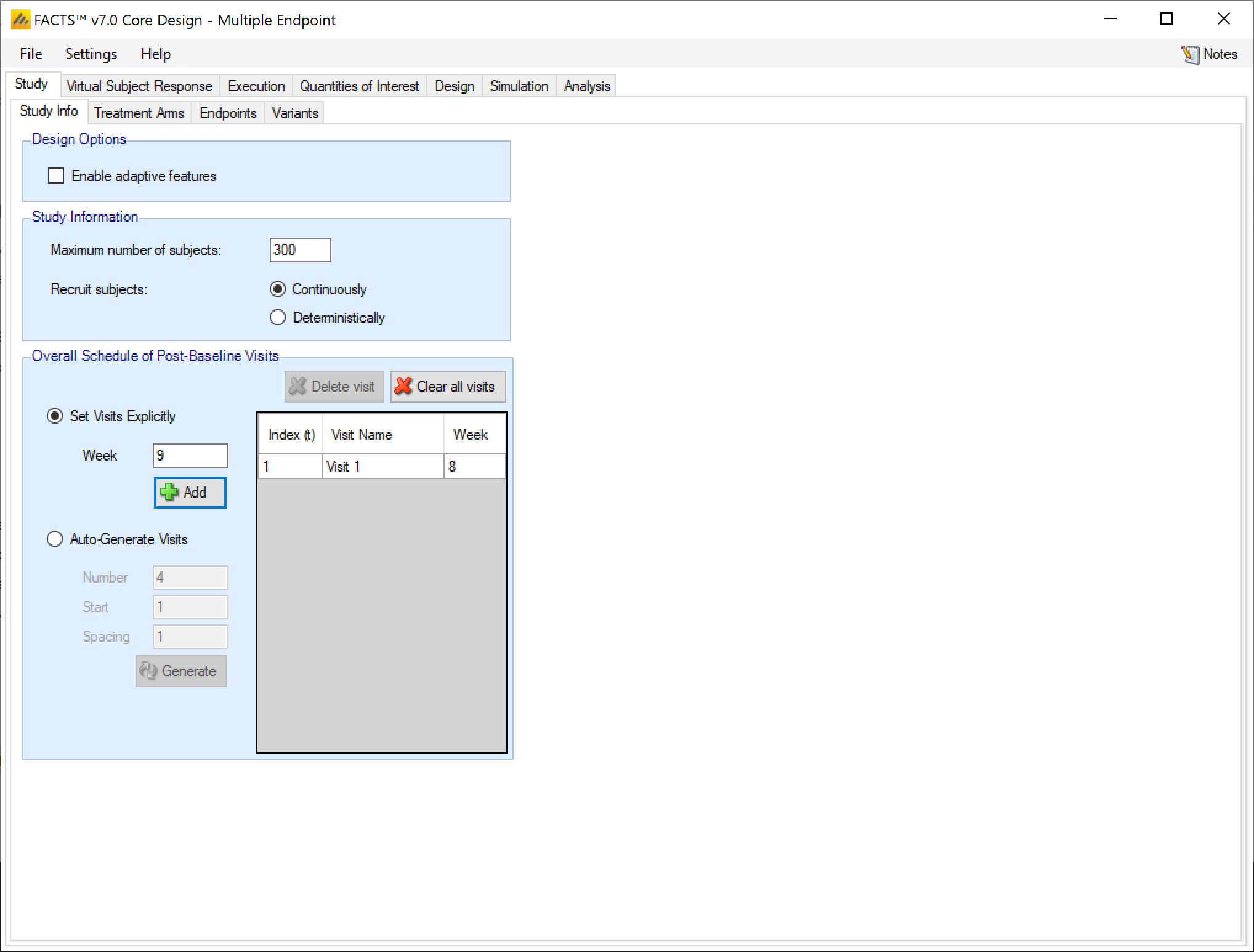
The study tab is simpler for multiple endpoint than it is for other FACTS Core design engines (Continuous, Dichotomous, or Time-to-event). Some options that are endpoint specific have been moved to the Endpoints tab, which only exists in the multiple endpoint engine.
Design Options:
In the design options section of the Study tab the user gets a check box for whether they want to enable adaptive features or not. Endpoint specific choices about using longitudinal modelling or special longitudinal options are moved to the Endpoints tab.
Enable adaptive features
Specify whether the design is adaptive or fixed. If “adaptive features” are enabled, some adaptive specific parameters and tabs are added to the GUI, such as the tabs for defining interims, early stopping criteria, and adaptive allocation.
Study Information:
The study information section allows the user to specify how many subjects to accrue and how subject accrual should be simulated.
Maximum Number of Subjects
Specify the maximum number of subjects that can be enrolled in the trial. Adaptive designs may stop sooner than this value, but no simulation can ever go past it.
Recruit Subjects
In multiple endpoint, subject accrual can only be done continuously or deterministically.
If recruited continuously, the user recruitment will be simulated stochastically with a Poisson process, using the parameters specified on the Execution > Accrual tab.
If recruited deterministically, the user specifies the recruitment date of every subject recruited by uploading a file of dates on the Execution > Accrual tab.
Overall Schedule of Post-Baseline Visits
The overall visit schedule is specified here. It’s called the “overall” visit schedule in the multiple endpoint engine because the visits entered here make up the set of all visits where any of the endpoints can be observed. When the details of the different endpoints are entered on the Endpoints tab, you will be able to specify which of these visits each endpoint is observed at and which visit will be the final observation for that endpoint.
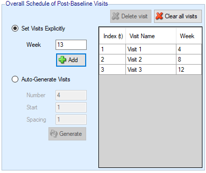
Visits can be specified one at a time by entering the required week value for the visit and then clicking ‘Add’, or by specifying a regularly spaced sequence: select ‘Auto-Generate’, enter the number of visits, the week of the first visit and the number of weeks between each visit and then click ‘Generate’.
Individual visits can be deleted by selecting them in the list and clicking ‘Delete’. The default visit names can be edited by clicking the visit name and typing. The week and the index cannot be changed. Should it be necessary to change the week of a visit, the incorrect visit must be deleted and a new one with the correct week number added.
Treatment Arms
As with all FACTS Core engines, the Treatment Arms sub-tab provides an interface for specifying the various dose levels, Control and Additional Comparator arms, and whether using a 2D treatment arm model.
The user may add doses either explicitly or by auto-generation.
The index column provides the ordering of the doses, as well as the number that will be used to subset the dose in dose response models and FACTS output. The dose name column is editable by the user, and is used to identify the doses in the VSR tab as well as in the simulation output shown on the Simulation tab. Effective Dose Strength (\(v_d\)) are the relative strength values of the doses, and are the values used in the dose response model analysis as \(v_d\). They have no units, but the proximity of doses to other doses will determine them amount of information sharing that occurs between doses in certain dose response models. Dose levels may not be edited directly – to change a dose level, delete the entry and add a new dose with the correct level.
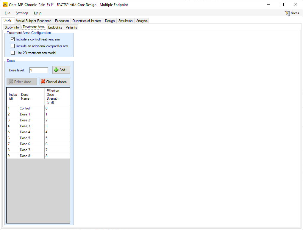
If “Include a control arm” is selected at the top of the Treatment Arms tab, then a control will be included in the table. Including a control arm causes many default QOIs to compare to control and sets frequentist tests, predictive probabilities, and conditional power to compare against the control arm rather than an OPC, among other things.
The active comparator arm can be compared against in posterior probability QOIs, and is always modelled independently in the dose response model.
2D Treatment Arm Model
If the user checks the “Use 2D treatment arm model” option, the screen changes to allow the treatment strengths to be specified on 2 axes, and to specify which of the treatment combinations thus created will actually included as arms in the trial.
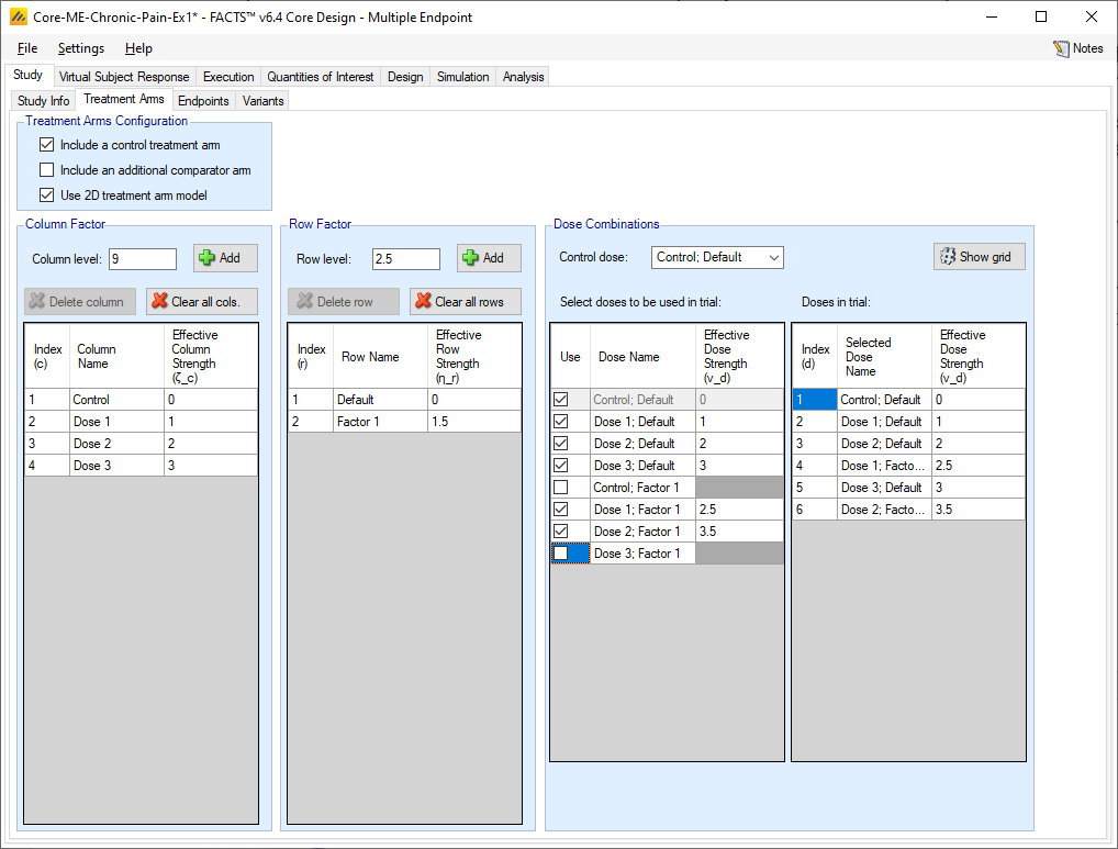
The user now specifies strengths as “Column Factors” and “Row factors”. For example, the Column factors could be different dose strengths and the row factors could be different dosing regimens, or different treatments that the investigational treatment could be combined with. Because of the way the factors are shown in FACTS graphs it is better to use the factor with the greater number of values as the column factor. From the point of view of the analysis however the factors are treated symmetrically. In FACTS we have adopted the neutral term “factor” to avoid the impression that these designs can only apply to doses and dosing regimens.
FACTS then shows all the potential combinations of column and row factors in the list “Select doses to be used in trial” in which the user selects which of the factor combinations that will be present as arms in the trial. FACTS constructs the “effective strengths” opf the combinations by simply adding together the strengths of the two factors, but while the strengths of the factors (like the strengths of “doses” in the 1D setting) cannot be simply changed (because of the problems of managing the ordering of the factors), strengths of combinations can be directly edited, and indeed must be edited to resolve any “ties”. All combinations must have unique strengths so that they can be ranked in order.
If a control treatment arm is included in the trial then a “Control” factor is included in the Column factors and the user selects which combination of this factor and a Row factor is the Control combination. This combination is given the effective strength 0 and moved to the head of the list of doses. If the “include a control treatment arm” option is checked, there must be a combination that acts as control dose. If the option is not checked there will be no control dose.
FACTS displays the resulting ordered list of combinations in the “Doses in trial” column.
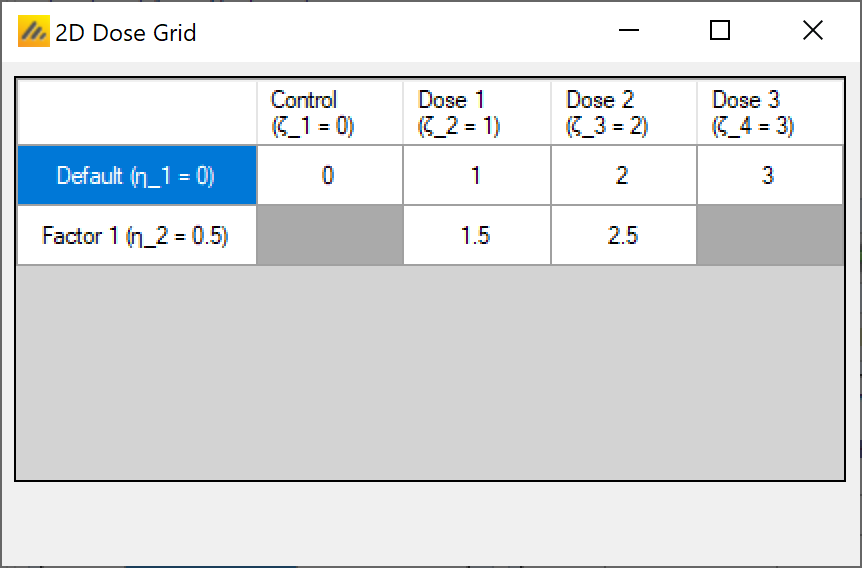
There is also a “Show grid” option that will display a small graphic of the 2D layout of these “Doses in trial”:
Endpoints
The Endpoint sub-tab allows the user to specify the nature of each endpoint, the target characteristics, and a utility function that allows the estimate of the response on the different endpoints to be combined into an overall utility.
Create Endpoints
The small table on the middle-left side of the screen allows for the creation of up to 4 endpoints. The name of each of the endpoints can be changed in the table by clicking on the entry. The order of the non-first endpoints can be changed by clicking on an endpoint and then clicking on the up or down arrows to the right of the table.
For each endpoint, the Endpoint Properties section allows for the endpoint specific characteristics to be supplied.
Endpoint Properties
Continuous Endpoints
For continuous endpoints, the first value provided is whether a higher response is subject improvement, or if a lower response is subject improvement.
Then, you select whether to simulate a baseline value for subjects. If yes, then specify whether the VSR (Virtual Subject Response) will be specified as a change from the baseline value or as a standalone final endpoint value.
Next, specify whether to use longitudinal modeling for this endpoint. If the “Use longitudinal Modeling” option is checked, then select one or more visits that subjects will observe this endpoint at. If not using longitudinal modeling, then select which visit is considered the final observed value for this endpoint. Each endpoint can have its own visit schedule, as long as those visits are included as part of the overall visit schedule on the Study Info tab.
Dichotomous Endpoints
For dichotomous endpoints, the first value provided is whether an observed response is a positive outcome or a negative outcome.
Next, specify whether to use longitudinal modeling for this endpoint. If the “Use longitudinal Modeling” option is checked, then the user can decide if they would like to use the restricted markov model to simulate longitudinal data or the standard transition matrix method. If using the restricted Markov model, specify whether subjects that reach the end of their follow-up without going to either absorbing states should be considered a success or a failure. Then, select one or more visits that subjects will observe this endpoint at.
If not using longitudinal modeling, select which visit is considered the final observed value for this endpoint. Each endpoint can have its own visit schedule, as long as those visits are included as part of the overall visit schedule on the Study Info tab.
Utility Function
The Multiple Endpoint design engine allows clinical trials to be designed and simulated where the within-trial and end-of-trial decisions can be based on multiple endpoints by using a composite score, or utility, derived by combining the different endpoint estimates. The utility function approach is incredibly open-ended and flexible, able to cope with different types of endpoints, different endpoint scales and different endpoint interrelations.
The utility function approach has two stages:
First, each endpoint is converted to its own utility score for each dose.
Then, the endpoint specific utilities are combined into a single overall utility for each dose.
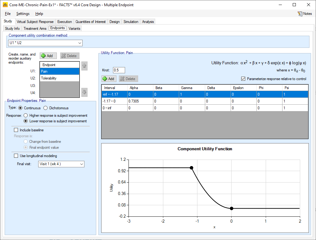
Each endpoint has its own utility function, as described above. Utilities are flexible piecewise functions of the estimated response for the endpoint.
First use the “Add” button to add the knots of the utility function – these are the segment boundaries in the range of the endpoint measure where different functions will be specified in each segment. For each segment created by adding a “knot” a row is created in the table, allowing the user to specify the coefficients of the utility function in that segment specifically.
The components of the utility that can be weighted based on their coefficients are: fixed, linear, quadratic, exponential, and log terms.
The coefficients that can be specified are:
Alpha: the coefficient of the quadratic term
Beta: the coefficient of the linear term
Gamma: the coefficient of the fixed term
Delta: the coefficient of the exponential term
Epsilon: the coefficient of x in the exponential term
Phi: the coefficient of the log term
Psi: the coefficient of x in the log term
Finally, the user specified whether the \(x\) in the utility function is relative to control or not. If the “Parameterize response relative to control” is checked, then \(x=\theta_d - \theta_0\) for a continuous endpoint, and \(x = P_d - P_0\) for a dichotomous endpoint. If the “Parameterize response relative to control” is checked, then \(x=\theta_d\) for a continuous endpoint and \(x=P_d\) for a dichtomous endpoint.
For a continuous endpoint, the utility function is defined on the range of \(x \in (-\infty, \infty)\). For dichotomous endpoints, if \(x\) is relative to control, then the utility is on the range \(x \in (-1, 1)\), and if \(x\) is not relative to control, then the utility is on the range \(x \in (0, 1)\).
It is not the intention that all, or even most, of the available coefficients are used in any one segment, typically only one or two are. The different terms are provided so that the required form can be selected for each segment – flat linear, quadratic, exponential or log. The default values of the coefficients are set so that only the linear component of the utility contributes.
Estimation of Utility in FACTS
An important aspect of the way FACTS estimates utility is that it estimates a probability density for the utility within the MCMC sampling. That is, the utility is calculated for every parameter sample within the MCMC, and the final distribution of the utility is based on those samples just like the estimates for the model parameters.
Each dose has a distribution of utility scores - not a single value. The utility is not estimated from the mean estimates of the dose response from the different endpoints.
This has some notable effects on the estimates of utility. If, for example, the utility function is a step function – for example if its value is 1 for response rates below a threshold and 0 above – as the estimate of the response rate will have some uncertainty then when the mean response estimates are around the threshold value, the estimate of utility will be between 0 and 1, based on the proportion of MCMC samples the fitted response rate was below the threshold. Indeed, the utility can be interpreted as the ‘probability the response rate is below the threshold’, and thus be useful or even exactly what is required.
Similarly, any utility function that has a floor or ceiling will result in a bias in the estimate of the utility to be above the floor or below the ceiling. – because in the distribution of the values for the utility the lowest the value can be is the floor and the final estimate of the utility would only be at the floor if all the values for the utility sampled in the MCMC were at the floor. Another effect of utilities with a floor or ceiling is that the estimate of the mean utility has a smaller standard error the further the value of the estimate of the mean of the underlying response is from an inflexion point (or “knot”).
These are not errors, nor does it mean utility functions with steps, ceilings or floors should be avoided, but these artefacts need to be understood – particularly when graphs of the estimated utility and the true utility are compared.
FACTS’ utility is based on the estimates of the response on each endpoint in each treatment arm. It is not the utility of outcome for each individual that would be a composite score and an endpoint in itself. To use that kind of utility, simulate the external subjects and their scores outside of FACTS using a program or script and calculate the composite score for each individual and write the results to a file in FACTS external virtual subject response format, this can then be used to drive simulations in FACTS of trial designs using that composite score. This might be a single endpoint (FACTS Core Continuous) design, or a Multiple Endpoint design, with the Composite score as the primary endpoint and up to 3 of the component scores as auxiliary endpoints.
In this latter case, the design would probably be making decisions based solely on the composite score (so the utility based criteria are unused), and FACTS Multiple Endpoint’s result summarization and charting is used to understand how when different responses are simulated on the component scores this translates into the composite score and the likely trial results.
Calculation of Arms’ probability of having the greatest utility
Like other probabilities in FACTS this is calculated during the MCMC sampling – the probability that an arm has the greatest probability is based on the proportion of MCMC samples when that arm had the greatest utility. It is not estimated from the utility of the mean estimates of the dose response for the different endpoints.
In any given sample if several arms have the same maximum toxicity, the arm with the lowest dose strength is selected. This is particularly useful when using dose response models with plateau features (the Plateau and U-shaped models). It means that where the utility is driven by this model, the arm that will be ranked most likely to have the greatest utility will be the one that lies at the start of the flat maximum response section. However it has a less desirable effect when the overall utility is formed by multiplying the utilities of individual endpoints and one of the endpoint utility functions has a segment where the utility is 0.
Component Utility Combination Method
In order to derive the overall utility score for a dose we first need to decide how the different utilities are to be used how they are to be combined.
At the top of the Endpoint tab is a control that is displayed regardless of which endpoint is being specified. It allows the formula to be selected that defines the values of the individual utility scores for each endpoint are to be combined to form the overall utility. The only operators supported are addition and multiplication, but all logically distinct combinations (given that the user can re-order the auxiliary endpoints) are provided:
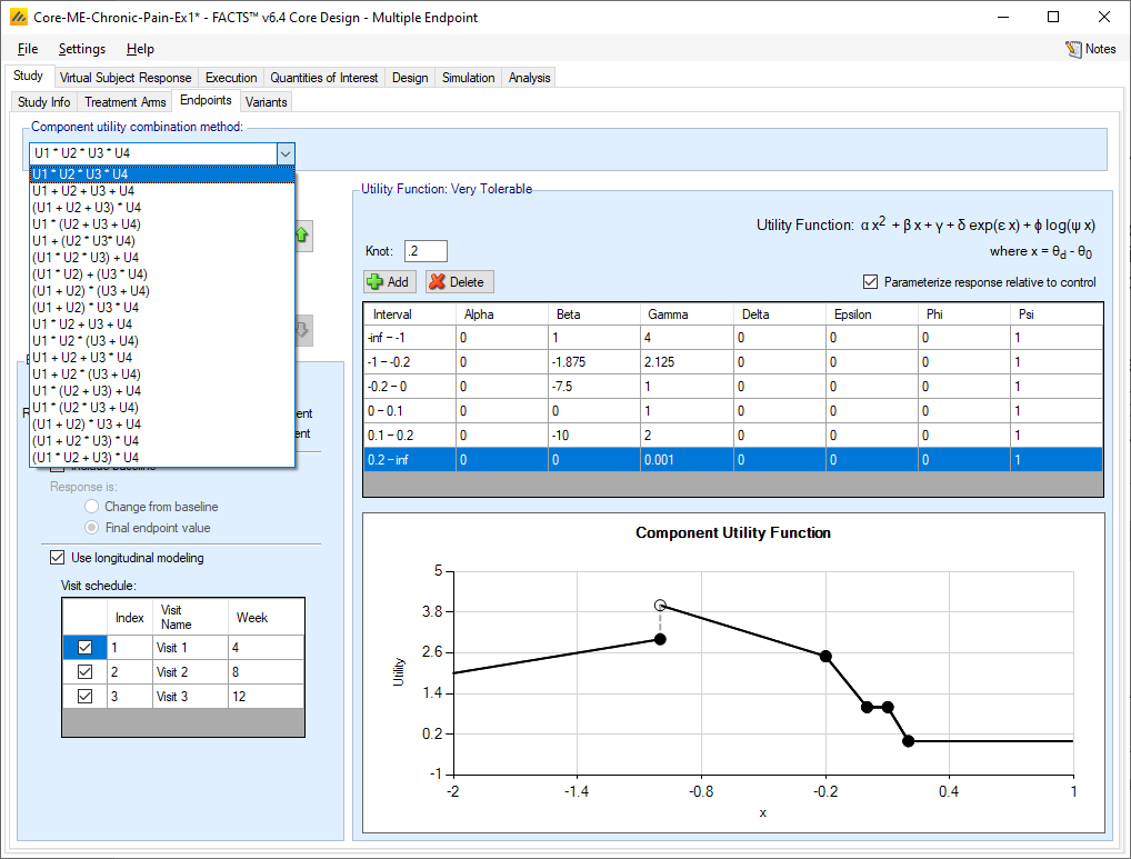
Utilities can be combined by multiplying them together or adding together, so when there are just two endpoints there are just two methods of combination: U1 + U2 and U1 * U2. With more endpoints there are more possible combinations. These allow utilities to be formed for a number of circumstances:
One efficacy and one safety/tolerability endpoint, U1 * U2. Here the purpose of the combination is to scale back the efficacy score if there are safety or tolerability issues. At its simplest, the utility function of the safety / tolerability endpoint is defined so that the estimate of the probability of an adverse event or lack of tolerability is transformed to so the utility is 0 where the safety / tolerability is completely unacceptable, and 1 where it is completely acceptable, with possibly a transition region in between. The utility of the efficacy endpoint could be simply the value of the efficacy endpoint.
This is not intended to replace SAE monitoring and the withdrawal of treatments arms that are unsafe, the safety monitoring may be for indicators of potential safety problems when the drug is taken for a longer duration than can be studied, or it may be for tolerability issues that would give compliance problems, or acceptability problems given the other treatments available.
Some possible variants are: where current treatments have a level of unpleasant side effects, the utility of the probability of a side effect for our drug may be >1 for side effect rates below this. The utility of the efficacy outcome may be 0 below a certain floor efficacy and capped at a maximum above a ceiling efficacy, perhaps to stop undue weight being given to an outcome that this thought unfeasible or avoid a level of utility on the efficacy score that would yield an overall utility that would be judged viable at a poor (but not utility 0) level of safety / tolerability.
Two efficacy endpoints, U1 + U2. Here the purpose of the combination is to allow success if either the response on either endpoint is very good, or is quite good on both endpoints. Some care will be required to define the utility functions of the endpoints so that different combinations of efficacy correctly yield sufficient utility or insufficient utility.
An efficacy endpoint and a ‘necessary but not sufficient’ biomarker, U1 * U2. Here the purpose of the combination is to yield an overall utility of 0 if the biomarker is not observed at the necessary levels, otherwise the utility is driven by the primary endpoint that is observed much later. This allows early stopping for futility, arm dropping, or adaptive allocation away from arms with poor levels of biomarker, but for success to be determined only on the basis of the primary endpoint.
Utilities with more than two endpoints are usually some form of combination of the above, for example a primary secondary and secondary endpoint and a safety/tolerability endpoint: (U1 + U2) * U3.
Devising and agreeing upon utility functions with a clinical team is part art and part science (and possibly, part politics). Some have expressed the opinion that these methods could never be used in practice because it would be impossible to get agreement, but experience shows agreement is possible. Generally, the process followed is roughly as follows:
The team agrees how the endpoints will be combined and specifies some key utility points – at specific combinations of response at the different endpoints – for example:
If there were no observed side effects, what is the minimum level of efficacy that would be a useful drug?
If the maximum expected level of efficacy was observed, what is the maximum level of side effects that could be observed that would leave a useful drug
See “Dose-Finding Based On Efficacy-Toxicity Trade-Offs” by Thall and Cook (2004), for a description of such an elicitation process.
The statistician creates utility functions for the endpoints that yield the desired overall utility value at the specified points.
Using FACTS some simple trials are simulated and example simulated datasets and analyses are studied and reviewed with the team. The team is asked the question “Given the data that was simulated, (and the distributions they were simulated from) what do they think of the utility assigned to the treatment arms?”
The statistician adjusts the utility functions and iterates the process of simulating and reviewing with the team.
Once the team is happy with individual examples of how utility is assigned, a larger number of simulations can be run and the estimates of the operating characteristics considered and other aspects of the trials design considered.
Estimation of Utility in FACTS
An important aspect of the way FACTS estimates utility is that it estimates a probability density for the utility within the MCMC sampling. That is, the utility is calculated for every parameter sample within the MCMC, and the final distribution of the utility is based on those samples just like the estimates for the model parameters.
Each dose has a distribution of utility scores - not a single value. The utility is not estimated from the mean estimates of the dose response from the different endpoints.
This has some notable effects on the estimates of utility. If, for example, the utility function is a step function – for example if its value is 1 for response rates below a threshold and 0 above – as the estimate of the response rate will have some uncertainty then when the mean response estimates are around the threshold value, the estimate of utility will be between 0 and 1, based on the proportion of MCMC samples the fitted response rate was below the threshold. Indeed, the utility can be interpreted as the ‘probability the response rate is below the threshold’, and thus be useful or even exactly what is required.
Similarly, any utility function that has a floor or ceiling will result in a bias in the estimate of the utility to be above the floor or below the ceiling. – because in the distribution of the values for the utility the lowest the value can be is the floor and the final estimate of the utility would only be at the floor if all the values for the utility sampled in the MCMC were at the floor. Another effect of utilities with a floor or ceiling is that the estimate of the mean utility has a smaller standard error the further the value of the estimate of the mean of the underlying response is from an inflexion point (or “knot”).
These are not errors, nor does it mean utility functions with steps, ceilings or floors should be avoided, but these artefacts need to be understood – particularly when graphs of the estimated utility and the true utility are compared.
Calculation of Arms’ probability of having the greatest utility
Like other probabilities in FACTS this is calculated during the MCMC sampling – the probability that an arm has the greatest probability is based on the proportion of MCMC samples when that arm had the greatest utility. It is not estimated from the utility of the mean estimates of the dose response for the different endpoints.
In any given sample if several arms have the same maximum toxicity, the arm with the lowest dose strength is selected. This is particularly useful when using dose response models with plateau features (the Plateau and U-shaped models). It means that where the utility is driven by this model, the arm that will be ranked most likely to have the greatest utility will be the one that lies at the start of the flat maximum response section. However it has a less desirable effect when the overall utility is formed by multiplying the utilities of individual endpoints and one of the endpoint utility functions has a segment where the utility is 0.
Having segments of utility 0 for an endpoint, and calculating the overall utility by multiplying the component utilities will lead to segments of 0 in the overall utility. If in only a proportion of the MCMC samples all arms have a utility of 0, this will result in that proportion of the probability of being the arm with the maximum utility being placed on the arm with the lowest dose strength, which might be odd given the utility in the other samples. It can lead to counter intuitive and sometimes undesired adaptations, such as in the adaptive allocation of subjects between the arms.
The solution is to not use 0 for the segments of low utility, but a small value such as 0.01, the multiplication with the utility of the other endpoints will then not flatten them all to exactly 0, but retain the utility profile at attenuated values.
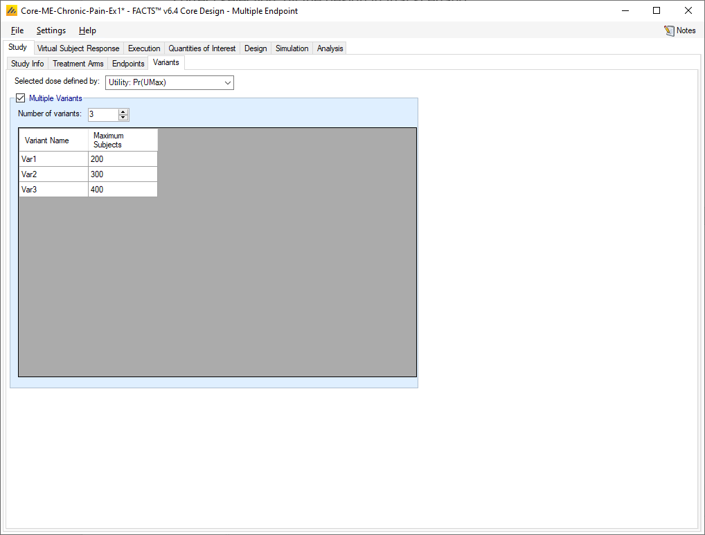
Variants
On this tab the user can specify that a number of design variants should be created. Currently, the only design feature that can be changed is the sample size (maximum number of subjects).
If “multiple variants” is checked, then the user can specify that simulations setups should be created for each simulation scenario with versions of the design with a different maximum number of subjects.
The user enters the number of variants they wish to create. Then in the resulting table, enter different “Maximum Subjects” for each variant. On the simulations tab FACTS will then create a copy of all the scenarios to run with each variant.