The continuous and dichotomous endpoints provide the ability to use longitudinal models to utilize data from incomplete subject’s observed early endpoint values. These subjects may be those that have dropped out, or subjects at an interim that have not had the opportunity to complete their follow-up.
The time-to-event endpoints also allow for using an early predictor endpoint to help in the estimation of the primary endpoint. The time-to-event predictor model works differently than the continuous or dichotomous longitudinal models. See here for a description of the time-to-event predictor models.
Multiple Imputation for Continuous/Dichotomous Endpoints
Unless a deterministic method is used such as LOCF or BOCF, longitudinal models inform the dose response estimates by using the longitudinal model to stochastically impute subjects’ final endpoint data when it’s not been directly observed.
To perform any longitudinal modeling, ‘Use longitudinal modeling’ must be checked on the Study > Study Info tab, and the subject visit schedule must be defined.
To include dropouts in the longitudinal analysis, on the Design > Dose Response tab select “Bayesian multiple imputation from post baseline.”
First, data from subjects with both intermediate and final observations is used to estimate the parameters of whatever longitudinal imputation model has been selected.
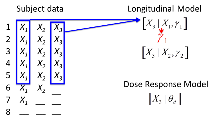
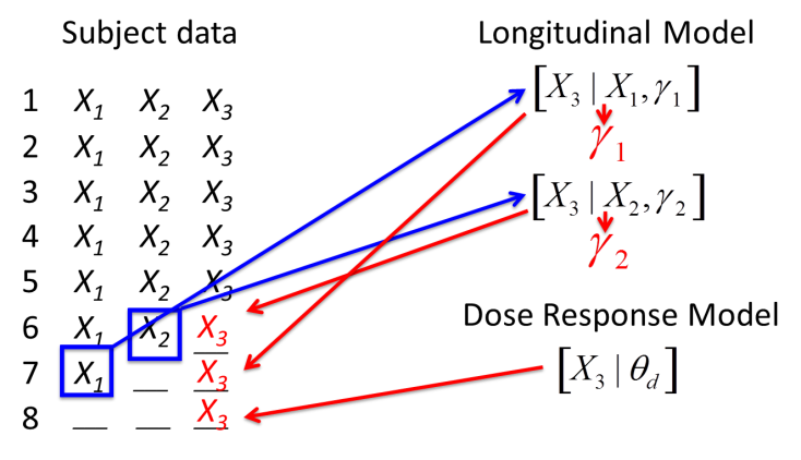
Subjects with missing final data have final data sampled from the posterior distribution of the longitudinal model given the subjects most recent intermediate visit (or in some models, all their available intermediate visit data). Subjects with no final or intermediate data have final data sampled from the posterior distribution of the dose response model given the dose arm the subject was allocated to.
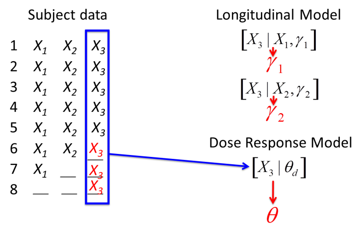
Once every randomized subject has either a real known final endpoint or an imputed final endpoint, the dose response model is re-estimated using that complete dataset.
This impute-then-fit-dose-response process is built into the MCMC estimation sampling loop. Each time we draw a new set of parameters from the longitudinal model they are used to impute the final endpoint of incomplete subjects. These subjects then inform the dose response model. Then we get a new sample from the longitudinal model and so on. The longitudinal models, with one exception The ITP model uses the current state of the dose response models in its imputation. , are not conditioned on the dose response models.
The missing final endpoint values are imputed with the uncertainty in the longitudinal model, and, as a result, the dose response model is estimated including both the uncertainty in the longitudinal model and the usual uncertainty in its parameters.
Above, it says “fit the dose response model,” as a step in the iterative process. The idea is that once you create a dataset through imputation you should update the dose response model MCMC chain until it converges. By default only 1 step is taken on the dose response model MCMC chain. It is safer, especially if doing a real analysis, to allow the dose response model parameter chains to converge slightly before imputing the missing data again. This can be done on the MCMC settings control on the Simulation tab and setting the “Samples per Imputation” parameter. As a rough guide, if it at some early interims > 5% of the data being analyzed will be imputed, a value in the range 2 to 10 is recommended to avoid underestimating the uncertainty. A higher number should be used the greater the proportion of imputed data.
A similar procedure is used when imputing event times based on a predictor endpoint in FACTS Core Time-to-Event.
FACTS is not fitting a joint Bayesian model of the longitudinal and dose response models. This would require a full MCMC fit of one model for every MCMC step of the other. Thus, if taking 2,500 samples, we would require a total of 2,5002 samples. This would make running simulations with longitudinal model prohibitively expensive.
How many longitudinal models?
When specifying a longitudinal model in FACTS, the user must clarify whether the longitudinal model is shared across all doses, or if different arms are to estimate different functions connecting early endpoints to the final endpoint.
The options that may be selected for the number of model instances are:
“Single model for all arms” – just one set of longitudinal parameters is estimated using all the subject data regardless of their treatment.
“Model control separately” – two sets of longitudinal parameters are estimated, one using data from just those subjects on the control arm, and the other using all the subject data from all the other arms.
“Model comparator separately” (only available if there is an active comparator arm) - two sets of longitudinal parameters are estimated, one using data from just those subjects on the active comparator arm, and the other using all the subject data from all the other arms (control and active treatments).
“Model control and comparator separately” (only available if there is an active comparator arm) - three sets of longitudinal parameters are estimated, one using data from just those subjects on the active comparator arm, one using data from just those subjects on the control arm, and the third using all the subject data from all the other arms.
“Model all arms separately” – a set of longitudinal parameters is independently estimated separately for each arm, each set estimated just using the data available from the subjects on that arm.
The fewer models used, the more data is pooled, the more precisely the model parameters can be estimated, and the more informative the intermediate data can be. Pooling data assumes that subjects in different groups have the same longitudinal profile, although they may still have different magnitude or probability of response (estimated by Dose Response Model).
If the response profile could be different on different treatment arms – for example, if subjects on control recover constantly over time, but those on an effective dose of the study drug recover very quickly early on, and more gradually later in their follow-up - a longitudinal model based on pooled data would tend to over-estimate the final endpoint of subjects on an effective dose of the study drug when only their early data was available. In a case like that, it would be better to use separate models. If the rapid early response was likely on all study drug treatment arms, then possibly use “model control separately.” If, however, the rapid response will only be seen on some study drug arms then use “model all arms separately”.
In addition to declaring how many longitudinal models should be estimated, when there is more than one model instance the user must declare if the prior distributions should be specified differently across each model instance or not. The options that may be selected for prior specification (for all LMs but linear regression) are:
- Same priors across all model instances
- Each instance of the model has identical prior distributions on its parameters. Estimation is still performed independently on each model instance.
- Specify priors per model instance
- Each instance of the model has its own priors that may vary across instances.
The linear regression longitudinal model has a different parameter set estimated for each visit, so its prior specification rules are slightly different. See the linear regression section below for specifics about prior specification specific to this model.