The Virtual Subject Response tab allows the user to explicitly define virtual subject response profiles, and/or to import virtual subject responses generated from an external response model.
Explicitly Defined
Baseline
This tab is present only if “Include baseline data” was selected on the Study Info tab.
Baseline profiles may be added, removed or renamed using the buttons and list on the left hand side of the screen. The baseline for each group is specified as a normal distribution, which may be truncated. If a truncated baseline is used, then samples will be drawn from the underlying normal and re-sampled if they fall outside the specified upper or lower bounds. [Note: clearly this will result in an observed baseline distribution with a different mean and SD from the underlying one].
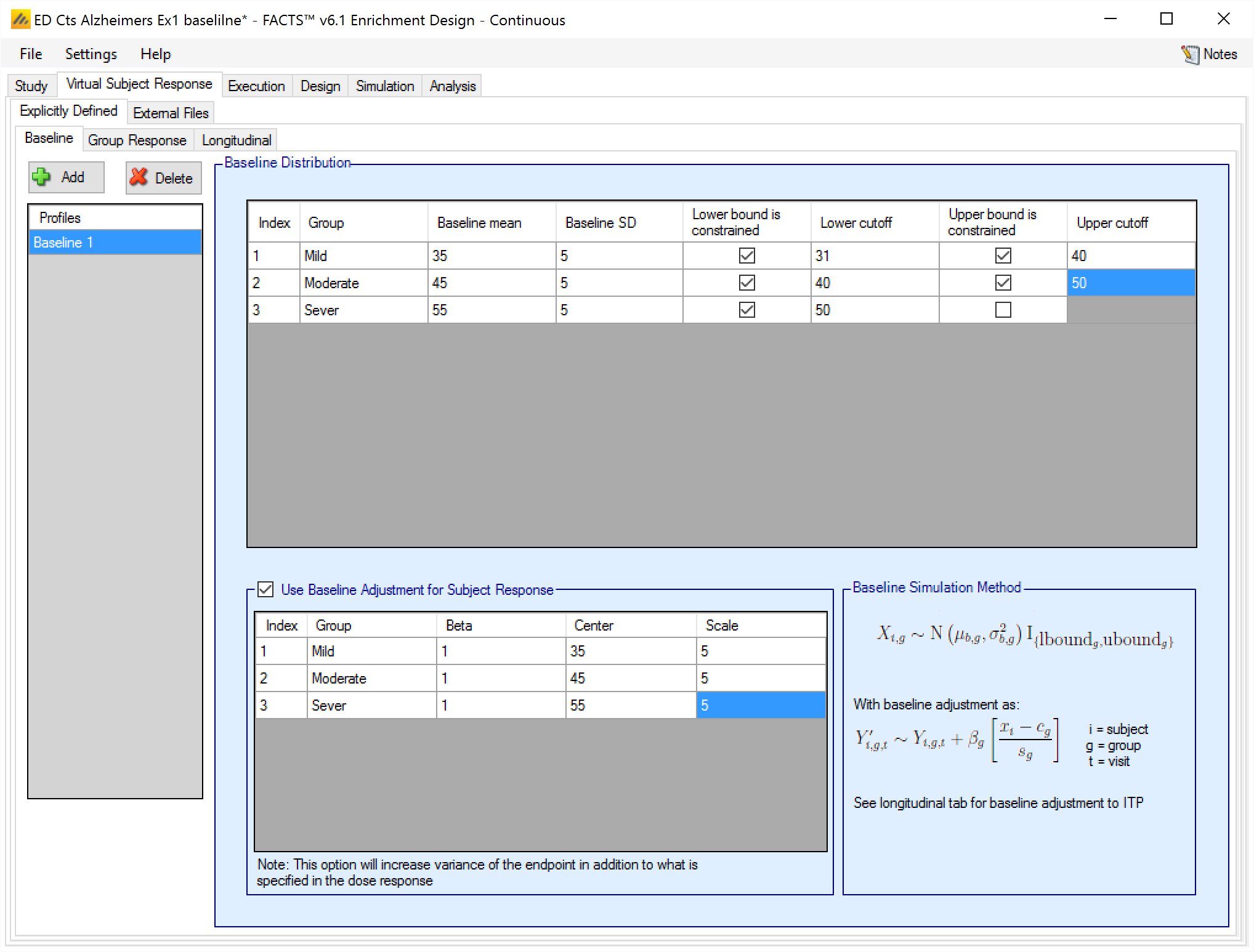
Optionally we can simulate a baseline effect on subject’s responses. This will be an adjustment to the “change from baseline” or “final endpoint value” depending on which definition of Response is being used.
If adjusting the final response based on baseline, then the user selects “Use Baseline Adjustment for Subject Response” and supplies 3 parameters for each group:
Beta - a coefficient that reflects the degree of influence of baseline on final score and the degree of variability in the final score due to baseline.
C – a centering offset, typically the expected mean of the observed baseline scores
S – a scaling element, typically set to the expected SD of the baseline.
Example – in the above screenshot for the severe group, a baseline of mean 55 and SD 5 has been specified – so a centering of 55 and scaling of 5 is used. Wishing to simulate an overall SD of 5 in the final change from baseline and apportion two-thirds the variance to baseline, Beta has been set as follows:
The desired final variance is 25 (52), divided between 2/3rd dose response and 1/3rd baseline effects.
The SD of the simulated response is set to 4.08 \(= \sqrt{\left( 25*\frac{2}{3} \right)}\)
The SD of the scaled baseline score is 1, so to contribute one third the final variance of 25, Beta is set to 2.89 \(= \sqrt{\left( 25*\frac{1}{3} \right)}\)
Note that when simulating a baseline effect in this way, limiting the range of baseline by specifying upper and lower cut-offs – which might be natural limits of the endpoint, or due to inclusion / exclusion criteria in the protocol – can significantly reduce the variance in the final endpoint due to the baseline effect.
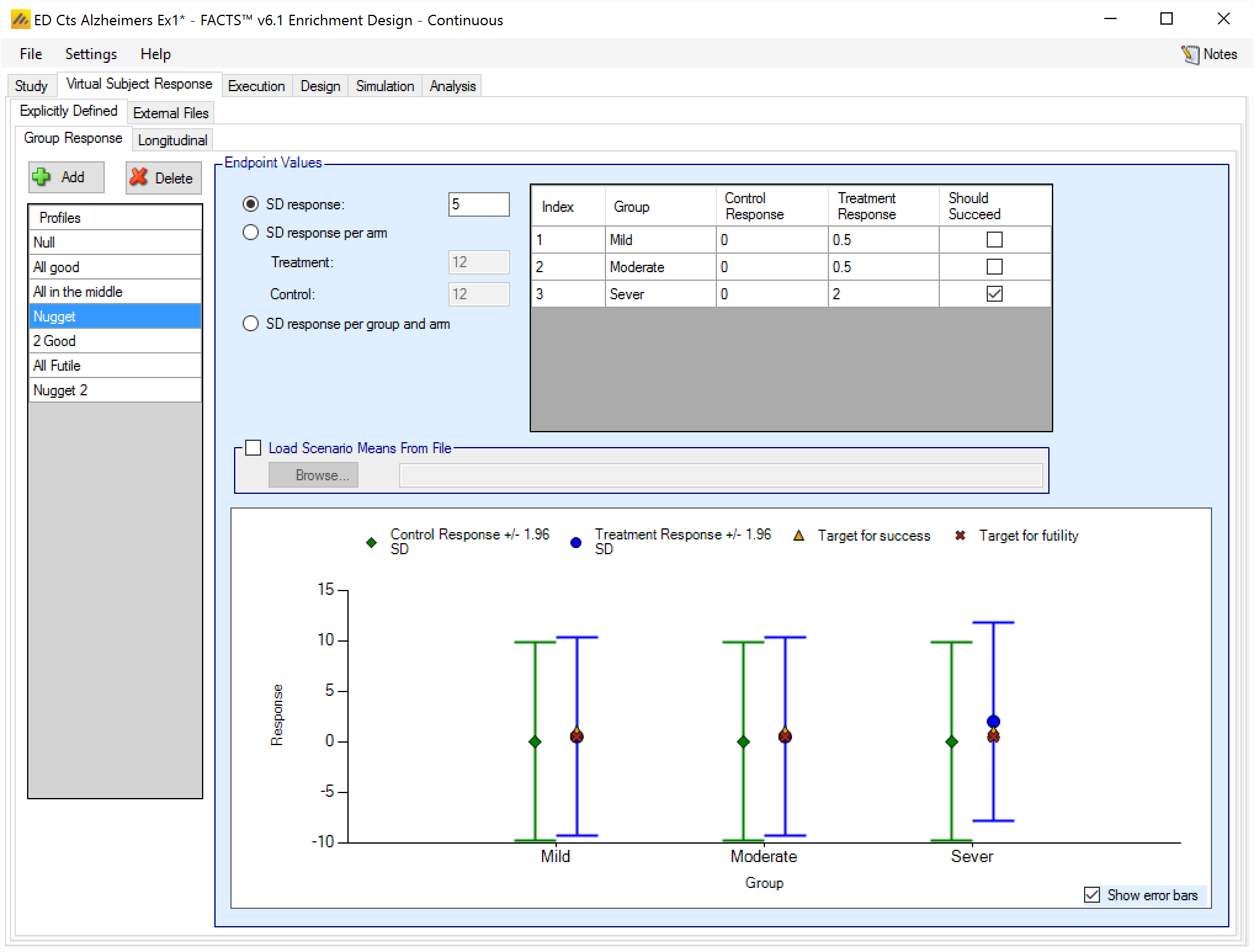
Group Response
Response profiles may be added, deleted, and renamed using the table and corresponding buttons on the left hand side of the screen in Figure 2. Mean response, the change from baseline (unless baseline is included in the simulation and the “Response is: Final endpoint value” option has been selected on the Study > Study Info, in which case the response simulated is the final endpoint value), values are entered for the treatment and control arms (if present) for each group directly into the “Treatment Response”/“Treatment change from baseline” and “Control Response”/“Control change from baseline” columns of the table. The graphical representation of these values updates accordingly.
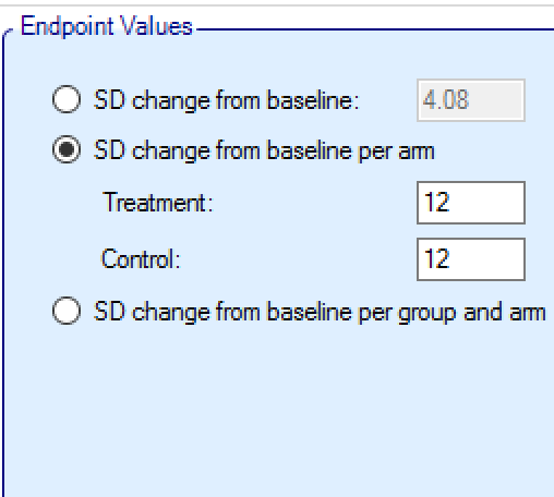
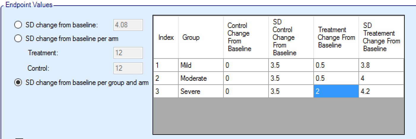
As well as the mean of each distribution to sample responses from, it is necessary to specify the variance, by specifying the standard deviation of the observations, termed here the ‘SD response’/‘SD change from baseline’.
The ‘SD response’/‘SD change from baseline’ needs to be specified for each profile, initially for each new profile it will be set to the default value, which is 12. It is very easy to overlook setting this value! If unexpected operating characteristics are seen for any response profile in ED, it is advisable to first check first that ‘SD response’/‘SD change form baseline’ has been set correctly for the profile before looking for more sophisticated reasons.
In addition it is possible for the user to specify if a group “Should Succeed” using the “Should succeed” checkbox on each row. This is then used in the summary of the simulation results to compute how often the simulated trial was successful and groups that ‘Should Succeed’ were successful (reported in the column “Ppn Correct Groups”) and how often the simulated trial was successful and groups that were not marked ‘Should Succeed’ were successful (reported in the column “Ppn Incorrect Groups”).
The graph that shows the response to simulate that has been specified – as with all graphs in the application – may be easily copied using the ‘Copy Graph’ option in the context menu accessed by right clicking on the graph. The user is given the option to copy the graph to their clipboard (for easy pasting into other applications, such as Microsoft Word or PowerPoint), or to save the graph as an image file.
Instead of specifying a single value for the SD of all responses, it is possible to specify (still on a per profile basis) a different SD for the responses for each of the treatment and control arms:
Or a different SD for treatment and control in each group:
Load Scenario Means From File
If the “Load scenario means from a file” option is selected then in scenarios using this profile the simulations will use a range of dose responses.
Each individual simulation uses one set of mean responses from the supplied file, each row being used in an equal number of simulations. The summary results are thus averaged over all the VSRs in the file. The use of this form of simulation is somewhat different from simulations using a single rate or single external virtual subject response file. When all the simulations are simulated from a single version of the ‘truth’ then the purpose of the simulations is to analyse the performance of the design under that specific circumstance. When the simulations are based on a range of ‘truths’ loaded from an ‘.mvsr’ file then the summary results show the expected probability of the different outcomes for the trial over that range of possible circumstances. Note that to give different VSRs different weights of expectation, the more likely VSRs should be repeated within the file.
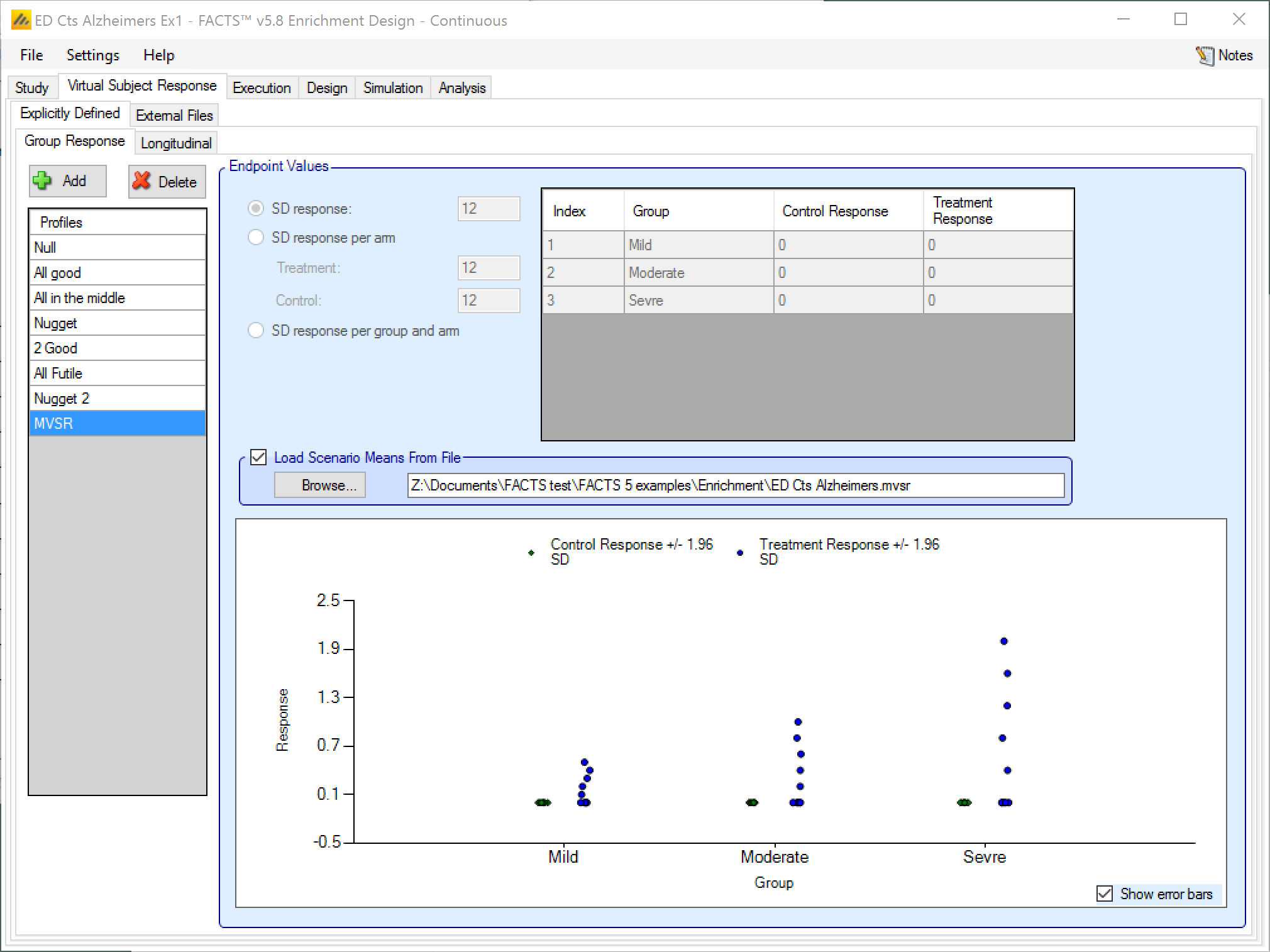
After selecting the “.mvsr” file the graph shows the individual mean responses and the overall mean response over all the VSRs.
The format of the file is a simple CSV text file. Lines starting with a ‘#’ character are ignored so the file can include comment and header lines. The format is:
If a control arm is being used: Each line should contain columns [MT1, MT2, … , MTG, ST1, ST2, … , STG, MC1, MC2, … , MCG, SC1, SC2, … , SCG] giving the true Mean responses and SD’s for the Treatment arm in each of the G groups, followed by the Mean responses and SD’s in the Control arms.
Without a control arm, using Objective Control: Each line should contain columns [MT1, MT2, … , MTG, ST1, ST2, … , STG] giving the true Mean responses and SD’s for the Treatment arm in each of the G groups.
For example:
# Alzheimer’s Example, 3 groups including control, SD of 5 for all arms
0.0, 0.0, 0.0, 5, 5, 5, 0.0, 0.0, 0.0, 5, 5, 5
0.0, 0.0, 0.0, 5, 5, 5, 0.0, 0.0, 0.0, 5, 5, 5
0.0, 0.0, 0.0, 5, 5, 5, 0.0, 0.0, 0.0, 5, 5, 5
0.0, 0.0, 0.0, 5, 5, 5, 0.0, 0.0, 0.0, 5, 5, 5
0.0, 0.0, 0.0, 5, 5, 5, 0.0, 0.0, 0.0, 5, 5, 5
0.1, 0.2, 0.4, 5, 5, 5, 0.0, 0.0, 0.0, 5, 5, 5
0.2, 0.4, 0.8, 5, 5, 5, 0.0, 0.0, 0.0, 5, 5, 5
0.3, 0.6, 1.2, 5, 5, 5, 0.0, 0.0, 0.0, 5, 5, 5
0.4, 0.8, 1.6, 5, 5, 5, 0.0, 0.0, 0.0, 5, 5, 5
0.5, 1.0, 2.0, 5, 5, 5, 0.0, 0.0, 0.0, 5, 5, 5
Longitudinal
If ‘Use longitudinal modeling’ has been checked on the ‘Study Info’ tab, and explicitly defined group responses have been specified, then it will be necessary to specify how to simulate the subjects’ responses at intermediate visits. This is done by selecting the correlation method to be combined with the response profiles to generate the intermediate results for subjects on treatment and control in all the groups.
The methods are parameterized so that their inclusion does not affect the mean and variance of the final endpoint to be simulated, and they scale automatically to suit each group response profile.
Three longitudinal methods are provided:
Correlated: is specified in terms of the ‘amount of noise’ carried forward from the last visit and the amount that is generated ‘a new’.
Hierarchical: visits are correlated through the use of a subject-specific random effect.
ITP: responses follow an exponential model over time with a subject specific random effect.
All methods allow the fraction of the final response and the fraction of the final variance observed at each visit to be specified.
Both methods can be parameterized across the whole trial or separately parameterized for each group.
Click here for an overview of longitudinal models for continuous endpoints in the FACTS Core engine.
Correlated Method
This method is defined by 3 values for each visit:
ft the fraction of the final mean response seen at visit t.
φt the fraction of the final sigma seen at visit t.
ρt the visit-to-visit correlation in the noise from visit t-1 to t.
The method can be parameterized for each group individually (as shown) or with one set of parameters for all groups.
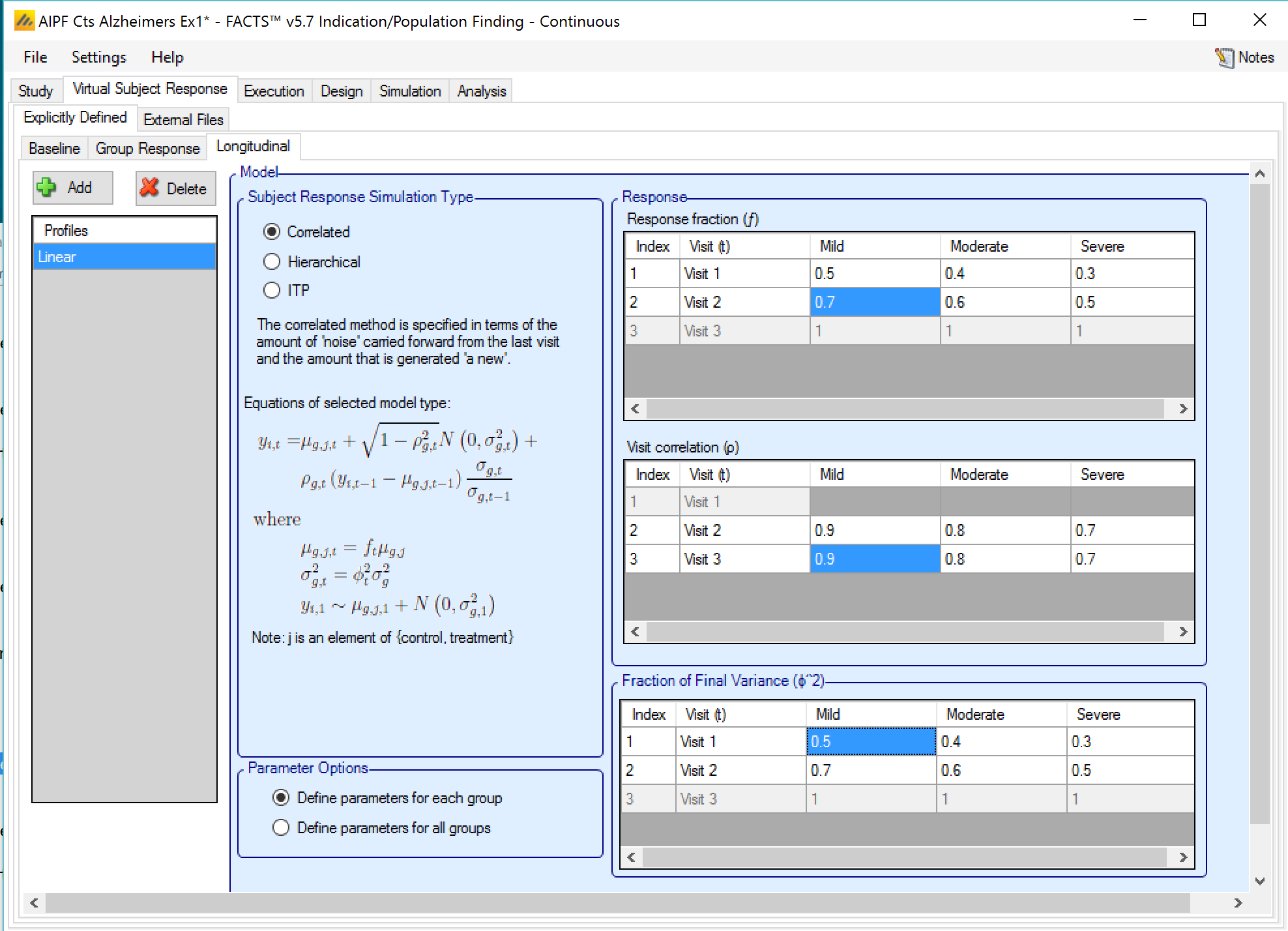
The equations currently use a subscript of ‘1’ for the first visit, corresponding to the values shown for the index of each visit shown in the table where the values are entered.
For the first visit, for a subject in group g, treatment arm a, the mean response is given by: \(\mu_{g,\ a,1} = f_{1}\mu_{g,a}\),
and the observed variance by \(\sigma_{g,a,1}^{2} = \varphi_{1}^{2}\sigma_{g,a}^{2}\)
thus the expected response \(y_{g,a,1}\) for a subject is \(y_{g,a,1} \sim\mu_{g,a,1} + N\left( 0,\sigma_{g,a,1}^{2} \right)\)
Where the final mean \(\mu_{g,a}\), and variance \(\sigma_{g,a}\), are as defined on the group response tab.
For the second visit, the mean response is given by: \(\mu_{g,a,2} = f_{2}\mu_{g,a}\),
and the observed variance by \({\rho_{g,1}\left( y_{i,1} - \mu_{g,a,1} \right)\frac{\sigma_{g,a,2}^{2}}{\sigma_{g,a,1}^{2}} + \sqrt{1 - \rho_{g,2}^{2}}N\left( 0,\sigma_{g,a,2}^{2} \right)}_{}^{}\)
(where \(y_{i,1}\) is the observed response at the ith subject’s first visit response) thus the variance is \(\sigma_{g,a,2}^{2} = \varphi_{2}^{2}\sigma_{g,a}^{2}\) but made up of a component that has already been observed at the previous visit, scaled by the correlation factor and relative variance at the second visit compared to the first, plus a new suitably scaled random component.
Hierarchical Method
This method is defined by 2 values for each visit:
ft the fraction of the final mean response seen at visit t.
φt the fraction of the final sigma seen at visit t.
And an overall (or per group) fraction \(\nu_{g}\) for how much of the final variance is due to inter-subject variance.
The method can be parameterized for each group individually (as shown) or with one set of parameters for all groups.
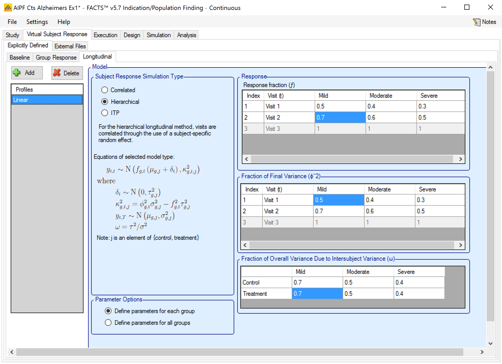
For the visit t, for subject i, in group g, treatment arm a
the expected response \(y_{g,a,t}\) for a subject is \(y_{g,a,t} \sim f_{g,t}\left( \mu_{g,a} + \delta_{i} \right) + N\left( 0,\kappa_{g,a,t}^{2} \right)\)
where \(\delta_{i}\sim N\left( 0,\tau_{g,a}^{2} \right)\)
and \(\tau_{g}^{2} = \upsilon_{g}\sigma_{g,a}^{2}\),
the variance of \(y_{g,a,t}\) will be \(\kappa_{g,a}^{2} + {f_{g,t}^{2}\tau}_{g}^{2}\), and \(\kappa_{g,a}^{2}\), will be set so that this \(= \varphi_{t}^{2}\sigma_{g,a}^{2}\)
Thus there is an inter-subject component to the variance \(\delta_{i}\), and an intra-subject component \(\kappa_{g,a}^{2}\).
ITP
This method is defined by 2 values:
k which controls how quickly the response changes with visit.
ν the fraction of the final variance that is independent of visit.
These values may be specified per arm or per group and arm.
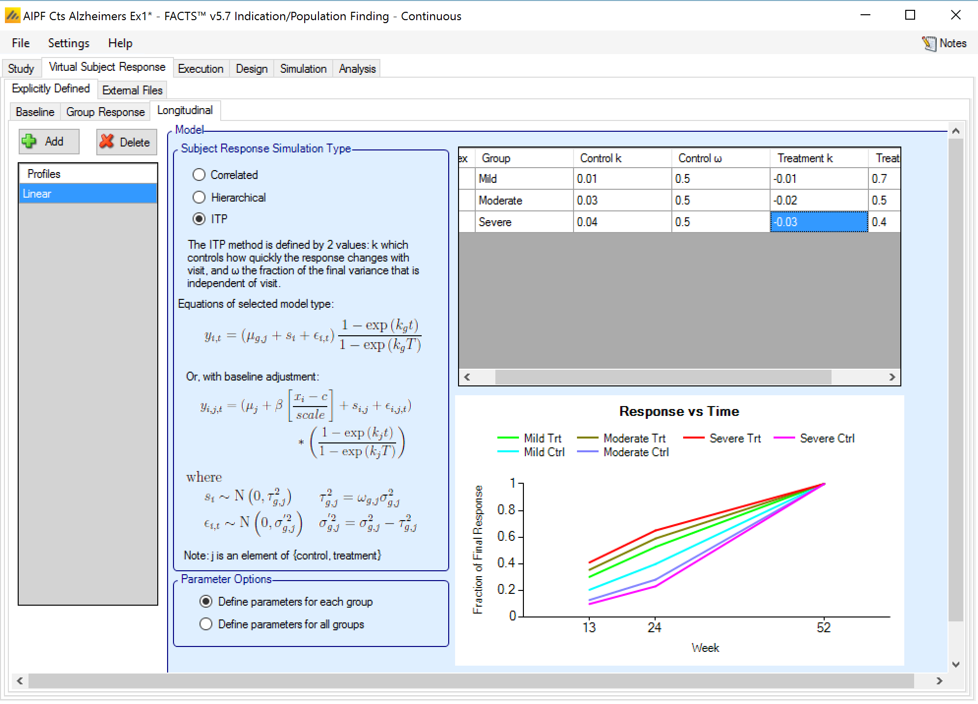
The subject variability σ2 as specified on the Group Response tab is divided into a per subject component, νσ2 and a component which varies between visits (1-ν)σ2.
The response for each subject (including both noise terms and any baseline adjustment term) is scaled at each visit as:
\[ y_{g,a,1} \propto \left( \frac{1 - \exp\left( kv_{t} \right)}{1 - \exp\left( kv_{T} \right)} \right) \]
where vt is the week of visit t and T is the final visit. The effect of some k values are shown below:
| K | Week 1 | Week 2 | Week 3 | Week 4 |
|---|---|---|---|---|
| -1 | 64% | 88% | 97% | 100% |
| -0.5 | 45% | 73% | 90% | 100% |
| 1 | 3% | 12% | 36% | 100% |
The later the final visit, the closer to zero interesting values of k will be, non-interesting values will be:
too +ve: the scaling factor is close to 0 until the final visit, or
too –ve and the scaling factor is almost 1 from the first visit onwards.
External
As well as simulating subjects’ responses within FACTS, they can be simulated externally, from a PK-PD model for instance, and imported into FACTS, and the supplied responses are sampled from (with replacement) to provide the subject responses in the simulation. The specification of a file containing subject response data (which must be in the required format) can be done from the External Files sub-tab depicted below.
To import an external file, the user must first add a profile to the table. After adding the profile, a file selector window is opened and the user must select the file of externally simulated data. To change the selection click the ‘Browse’ button.
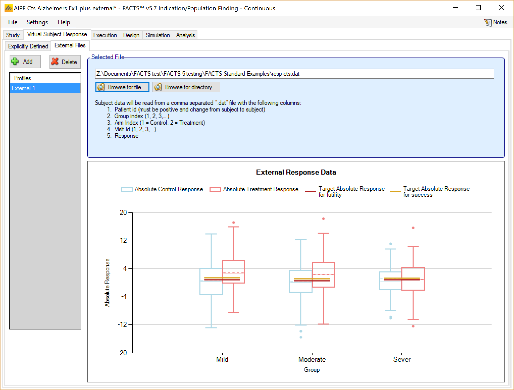
Required Format of Externally Simulated Detail
The supplied data should be in the following form: an ascii file with data in comma separated value format with the following columns:
Patient id (must be positive and change from subject to subject)
Group index (1, 2, 3, … )
Arm Index (1 = Control, 2 = Treatment)
Visit Id (1, 2, 3, …)
Response
The GUI requires that the file name has a “.dat” suffix.
The following shows values from an example file. Note that all visits for each subject must be grouped together. Thus all the data for the first subject comes before that of the second, and so on.
#Patient ID, Group Index, Arm Index, Visit, Response
1, 1, 1, 1, 0.5
1, 1, 1, 2, 0.8
1, 1, 1, 3, 1.2
1, 1, 1, 4, 0.9
2, 1, 2, 1, 0.4
2, 1, 2, 2, 0.6
2, 1, 2, 3, 0.8
2, 1, 2, 4, 0.9
3, 2, 1, 1, 0.45
3, 2, 1, 2, 0.55
3, 2, 1, 3, 0.6
3, 2, 1, 4, 0.5
Simulated subjects will be drawn from this supplied list, with replacement, to provide the simulated response values. The treatment response analysis in FACTS will be based on the values supplied – if you require the analysis to be on patients change from baseline, then you should supply change from baseline values as the subjects’ responses in the file. Conversely if the analysis should be on the absolute value of the response then these are the values that should be supplied as the subject’s response.
If baseline is included, each subject must include a visit 0 for the baseline, and the absolute values of the subject responses should be supplied, the option on the Study > Study Info tab to include baseline allows the specification of whether the analysis should be on
the absolute values,
or change from baseline values and FACTS will calculate these and perform the analysis on them. For example the above data might become ….
#Patient ID, Group Index, Arm Index, Visit, Response
1, 1, 1, 0, 6.2
1, 1, 1, 1, 6.7
1, 1, 1, 2, 7.0
1, 1, 1, 3, 7.4
1, 1, 1, 4, 7.1
2, 1, 2, 0, 5.4
2, 1, 2, 1, 5.8
2, 1, 2, 2, 6.0
2, 1, 2, 3, 6.2
2, 1, 2, 4, 6.3
3, 2, 1, 0, 6.9
3, 2, 1, 1, 7.35
3, 2, 1, 2, 7.45
3, 2, 1, 3, 7.5
3, 2, 1, 4, 7.4