In FACTS Core TTE, ‘predictor endpoints’ can be used in a similar way to early observations of the clinical endpoint measure in FACTS Core Continuous and Dichotomous. That is, they are used to inform the analysis about what the final outcome is likely to be for subjects for whom the final outcome has not yet been observed If a subject drop’s out, their final endpoint will never be observed, but their predictors are still used to impute the subject’s possibly final time to event if the predictor is observed before the dropout. . The estimates of the predictor response can also be used in QOIs, and thus somewhat like an additional endpoint and used for decision making.
The dose-predictor model is used to impute subjects’ predictor responses based on their treatment allocation when their predictor response has not yet been observed. The predictor-endpoint model is used to impute their time to final endpoint when that has not yet been observed.
The differences between predictor endpoints in FACTS Core TTE and early endpoints with longitudinal modeling in FACTS Core Continuous and Dichotomous are that:
There is only one observation of a predictor per-subject, there may be multiple early observations per subject of the clinical endpoint for use in a longitudinal model.
In FACTS Continuous and Dichotomous, longitudinal modelling is over time. There is no response modeling of early observations across doses, longitudinal modeling is either for different doses or pooled.
In FACTS TTE the design can include a dose-predictor model that
Allows subjects’ predictor event endpoint to be imputed (Imputation is described in the FACTS Core Design Guide).
Allows early stopping decisions to taken based on the estimates of the dose-predictor model.
For all predictor responses (\(Z\)) for time-to-event endpoints, the engine estimates both a marginal predictor distribution (normal mean and variance for continuous, probability of response for dichotomous, or a piecewise exponential hazard model for time to event predictors), and a working model relating the predictor to the final endpoint. The marginal predictor distribution is used to impute predictors for subjects lacking an observed predictor value, and may also be used for stopping (see section on stopping). The working model is used to impute final event times for subjects lacking a final endpoint. For subject missing both a predictor and final endpoint, the predictor is imputed first from its marginal distribution, and then the final endpoint is imputed conditionally on the predictor \(Z\).
Dose Response Model
Continuous & Dichotomous Predictors
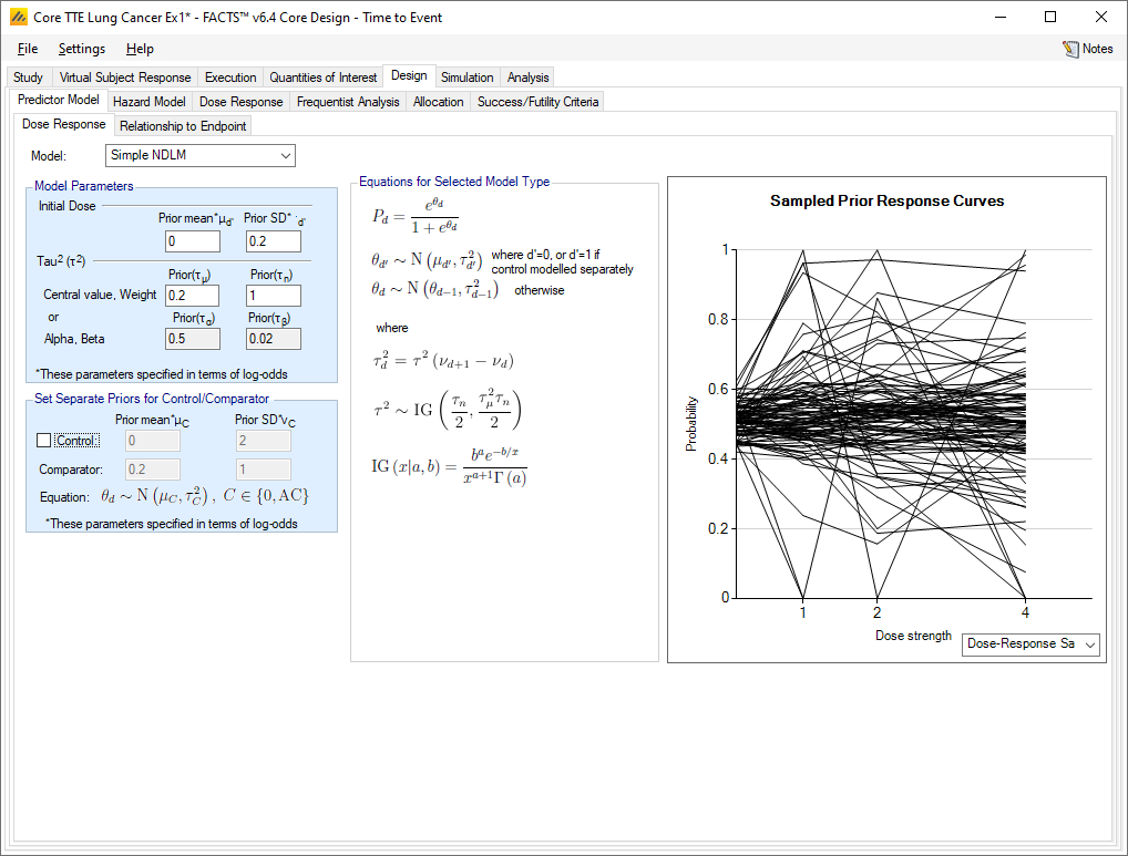
For the predictor model with a continuous or dichotomous predictor, there are two tabs within the Design > Predictor Model tab – the Dose Response and the Relationship to Endpoint tabs.
The dose response model for the predictor is the model used to estimate the marginal distribution of the predictor response at each dose as a normal mean and variance for a continuous endpoint or mean and variance of the log-odds for a dichotomous endpoint. The dose response options are as per the continuous and dichotomous endpoint standard dose response options (except that the use of BAC for the predictor is not supported). The predictor dose-response model can be selected and specified completely independently of the dose response model for the primary time-to-event endpoint (the model of the log hazard ratio).
Continuous Predictor
Within each dose (including control and active comparator), the marginal distribution of the predictor \(Z\) is a normal distribution with mean \(\theta_{Zd}\) and standard deviation \(\sigma_Z\). The standard deviation is common across the doses, but the means \(\theta_{Zd}\) are allowed to vary across the same range of doses based on the predictor’s dose response model. The dose response for the predictor does not need to match the dose response for the final endpoint, and the two models are estimated independently of eachother.
Dichotomous Predictor
A dichotomous predictor is handled similarly to a continuous predictor, with the predictor’s marginal distribution having its own dose response model. Like in the typical dose response model on a dichotomous endpoint when it is the primary endpoint, the dose response model estimates the log-odds of the response rate for each dose.
Time-to-Event Predictor
For the predictor model with a time-to-event predictor, there are three tabs within the Design > Predictor Model tab – the Hazard Model, Dose Response, and the Relationship to Endpoint tabs.
As in the response model for the primary event, the response model for a time to event predictor comprises a hazard model of the predictor for the event rate on the control arm, and a dose response model used to estimate the marginal distribution of the non-control dose predictor response for each dose as a normal log-hazard ratio.
The hazard model and dose response options for the predictor endpoint are similar to the hazard model and dose response options for the primary time-to-event endpoint, except that the use of the cox model or BAC for the predictor hazard model is not supported. The predictor dose-response model is selected, specified, and estimated completely independently of the dose response model for the time-to-event endpoint.
Relationship to Endpoint Model
On the Relationship to Endpoint tab, the user specifies the prior distributions for the relationship to endpoint model.
The relationship to endpoint model determines how the early predictor data impacts the primary time-to-event endpoint. After the dose response model for the predictor endpoint is calculated, the subjects with both a predictor value and a primary endpoint event are used to estimate the relationship to endpoint model, described below. Then, with this model calculated, all subjects who have a known predictor endpoint value, but do not have an observed primary endpoint event have their time to event imputed conditional on their predictor endpoint value.
It is possible to specify a minimum information (subjects with both predictor outcomes and final events) before the predictor model is used to impute time-to-event for subjects where their final event has not yet been observed. It also possible to disable the imputation completely, and simply have the predictor endpoint and final event be modelled separately.
Tips on Prior Strength and Informative Priors
If the main use of the predictor is to improve the information for the final analysis, unless the trial has a particularly small sample size, usually weak priors can be used so the model is driven by the data observed in the trial.
If the model is to be used to improve the information at interim analyses, and even at the first interim there will be some events observed to allow an initial model to be fitted (even though it might have a very diffuse posterior), again weak priors can be used.
If the model is to be used to allow interim analyses before any events are likely to have been seen, then informative priors are necessary.
When there is a need to set informative priors, one way to establish the values to use is to estimate them from simulations using external data file based on actual data.
Method
Create a simple, fixed trial with a sample size (per arm) of the weight of the prior desired, with non-informative priors for the predictor model.
Create an external file of actual data, or data sampled from the prior predictor-time-to-event model with at least as many samples per arm as the sample size in step 1.
Run 100 simulations and take the averages of the posterior estimates of the predictor model parameters to use as informative values in the actual design.
Continuous and Dichotomous Predictors
The relationship to endpoint model is:
\(T_{i} \sim \text{Exp}(\lambda_{d}\ e^{\beta Z_{i}})\) for a continuous predictor where \(Z_i\), is the observed value of the predictor for the \(i\)th subject
\(T_{i} \sim \text{Exp}(\lambda_{d}\ e^{\beta Z_{i}})\) for a dichotomous predictor where \(Z_i=0\) or \(1\) is the observed dichotomous predictor for the ith subject
That is, for the ith subject, the time to their event is taken to follow an exponential distribution with mean \(\lambda_d\ e^{\beta Z_i}\).
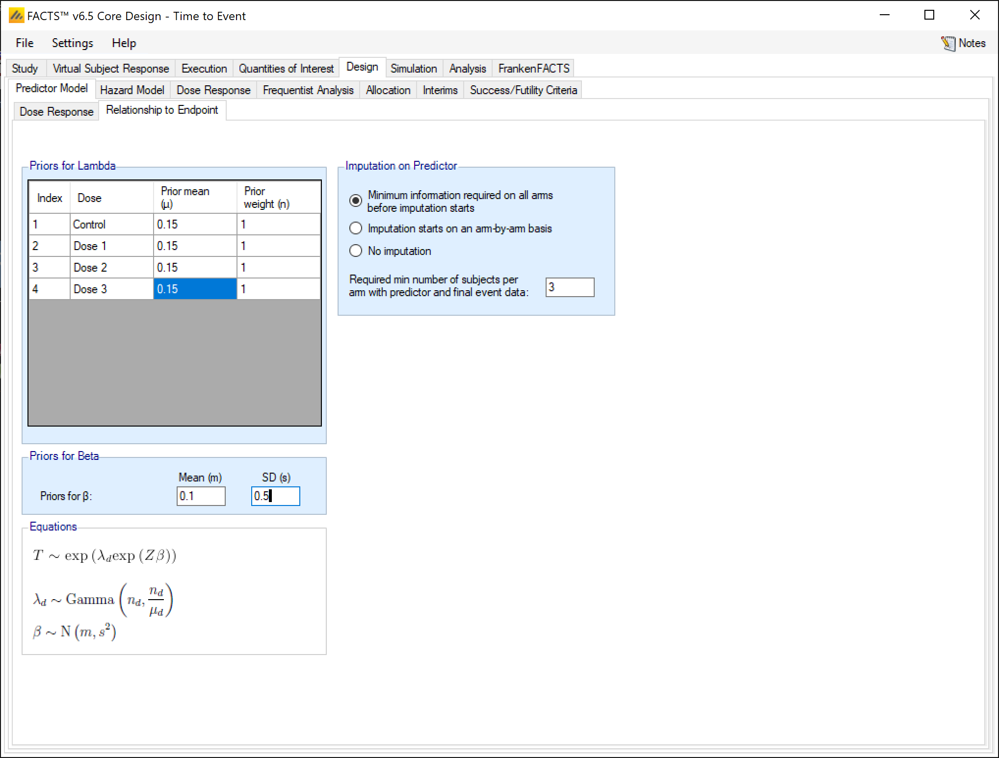
For both continuous and dichotomous predictors, the priors on the \(\beta\) and \(\lambda_d\) parameters are:
\[ \lambda_d \sim \text{Gamma}(\alpha_d, \beta_d) \]
\[ $\beta \sim \text{N}(m, s)\]
\(\lambda_d\) is esimated independently for all doses. The coefficient \(\beta\) does not have a subscript, because it is constant across all doses.
For the dichotomous predictor, we can simplify the notation of the relationship to endpoint model since \(Z\) can only be two different values (0 or 1).
\[T\mid (Z=0) \sim \text{Exp}(\lambda_d)\] and \[T \mid (Z=1) \sim Exp(\lambda_d e^{\beta})\].
For a continuous predictor, \(\lambda_d\) is the dose dependent hazard rate when the predictor is 0. For a dichotomous predictor \(\lambda_d\) is the dose dependent hazard rate when the predictor is 0. The \(\lambda\)s have independent gamma priors for each dose, specified by their expected mean and a weight in equivalent number of events seen. Thus, a weight of 1 would be very weakly informative with any normal number of events. A weight of 0.1 would be uninformative with even a small number of events. A way to think about the use of a weight of \(>1\) is, if weight of \(n>1\) is used, then after \(n\) actual events are observed the posterior mean estimate of \(\lambda\) will be the average of the observed mean and the prior mean.
The \(\beta\) parameter has a normal prior, specified by its prior mean and standard deviation. For a continuous predictor, this is the log scaling factor of the hazard rate for the correlation of the event rate to the predictor. For a dichotomous predictor, it is the log scaling factor of the hazard rate for subjects who have had response on the predictor. For a continuous predictor with the center and scale values set so that the value of \(Z\) will vary approximately between \(-1\) and \(1\), and a dichotomous predictor where the predictor value is \(0\) or \(1\), a prior distribution of \(N(0,5)\) for \(\beta\) would mean that \(e^{\beta Z}\) will take values between \(22,000^{-1}\) to 22,000 and the prior could be deemed to be essentially uninformative. Large values (>>5) for the SD of the prior for \(\beta\) can lead to numeric overflow in the simulator. If the values of Z do not largely fall in the range \([-1, 1]\), it is suggested that the prior for \(\beta\) be constructed to limit the coefficient \(\exp{(Z\beta)}\) to lie within its plausible range. If the prior for \(\beta\) is left uninformative and \(Z\) can take values \(>> 1\) it can result in inflation in the uncertainty in the estimates of the hazard ratios of subject’s time to final event from a few extreme imputed time-to-event values for subjects whose times-to-event are imputed, particularly if their predictor value is imputed too.
Time-to-Event Predictor
For the time-to-event predictor, the relationship to endpoint model is simply a per-dose hazard rate for the time from the predictor event to the final event. For each dose, the user specifies the parameters of a gamma prior distribution for this ‘post-predictor event’ hazard rate. This model is a simple exponential, not piecewise.
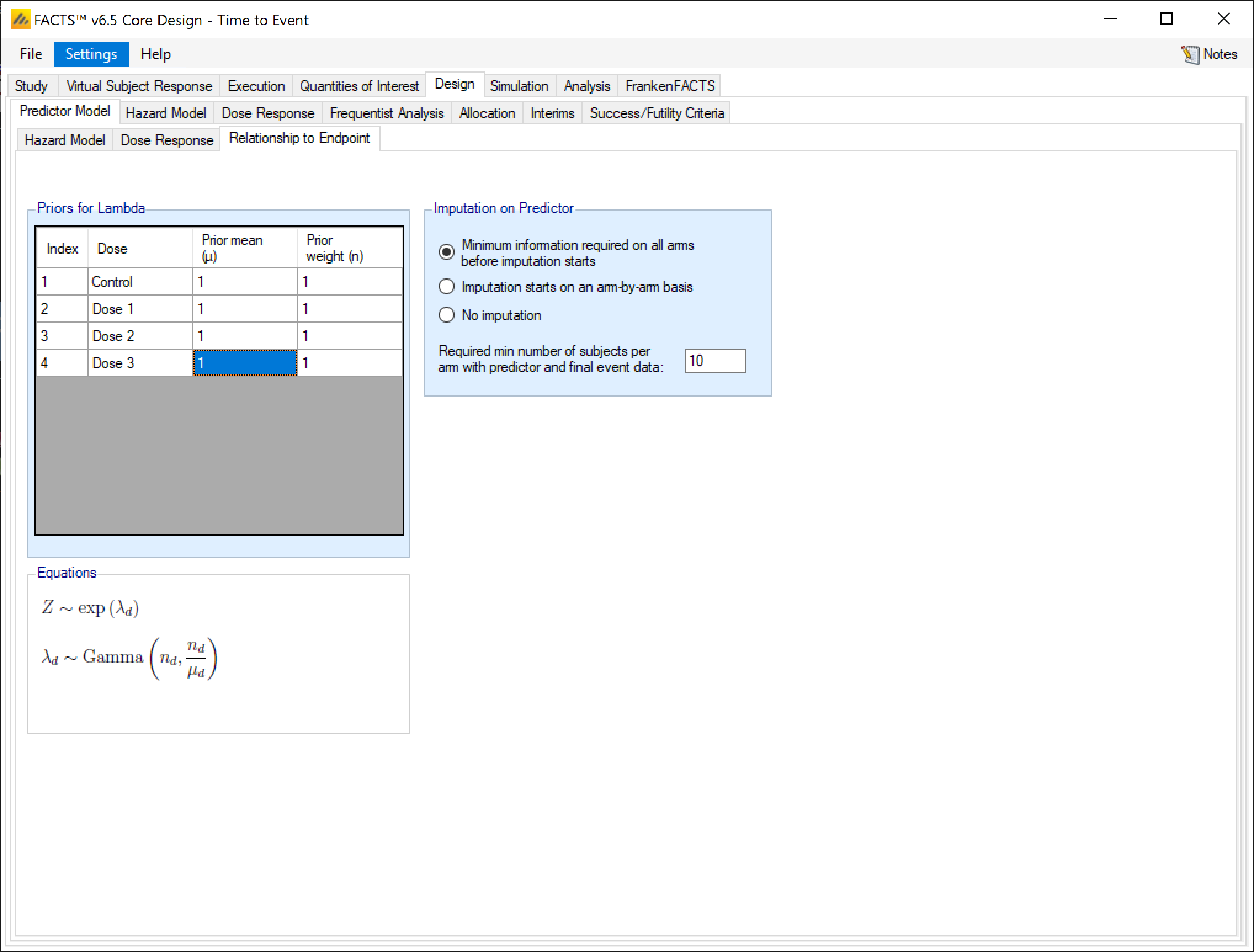
The time-to-event predictor is qualitatively different than the continuous or dichotomous predictors. Instead of the predictor adjusting the hazard, the time-to-event predictor is viewed as an offset. The final endpoint is viewed as a sum of a predictor time \(Z_1\) and a post-predictor time \(Z_2\), where \(Z_1\) and \(Z_2\) are independent random variables and the final endpoint is thus \(Z_1 + Z_2\).
For the relationship to endpoint model, \(Z_1 \sim PWExp(\lambda_{1s}*\theta_{1d})\) and \(Z_2 \sim Exp(\lambda_{2d})\), with priors \(\theta_{1s} \sim Gamma(\alpha_{1s}, \beta_{1s})\), \(\theta_{2d} \sim Gamma(\alpha_{2d}, \beta_{2d})\) (with \(Z_1\)’s control hazard model potentially being piecewise exponential).
For imputation of the primary endpoint event time, a subject missing both the biomarker and final endpoint times has both \(Z_1\) and \(Z_2\) imputed, with the final endpoint imputed as the sum of the two. For a subject with a predictor time but no final endpoint, \(Z_2\) is imputed and added to the observed predictor time to impute the final endpoint.