Dose response models in FACTS may be more accurately called final endpoint models. They create and model a relationship across the doses specified in the Treatment Arms tab. Often, but not always, the dose strength, called “Effective Dose Strength” in the Study > Treatment Arms tab of FACTS, is used in the dose response models to determine the order of doses, and which doses are more related to others.
The dose response models can be simple, and model the doses largely independently, as is done with the Independent Dose Model or the Independent Beta Binomial Model (dichotomous only). They can have logistic style models with interpretable parameters, like the 3-parameter logistic or the \(E_{max}\) model (called Sigmoidal in FACTS). The dose response model can also be a model that creates a smooth, spline like, model over the doses using a normal dynamic linear model (NDLM), a monotonic NDLM, or a 2nd order NDLM.
For all endpoints, we model the response at each dose, d, in terms of \(\theta_d\) on a continuous scale, allowing a consistent and rich range of dose response models to be used for all endpoint types. Transformations (see below) of the dichotomous and time-to-event responses are used to achieve this.
Continuous, Dichotomous, and Time-To-Event
With the exception of two dose response models specific to a dichotomous endpoint, the same dose response modeling facilities are available for all endpoints.
Let there be D total doses including the control arm if it exists. For any endpoint, the estimate of dose response model is called \(\theta_d\) for a dose \(d \in \{1, \ldots , D\}\).
In the continuous dose response models the individual response or change from baseline (if it is being used) \(Y_i\) of the \(i^{th}\) subject allocated to dose \(d_i\) is modeled: \[ Y_i \sim \text{N}(\theta_{d_i}, \sigma^2) \]
The dose means \(\theta_{d}\) have formulations depending on the selected dose response model.
The variance \(\sigma^2\) has an inverse-gamma prior. For a description in how FACTS elicits parameterizations for the Inverse Gamma distribution, see here.
In the dichotomous case the final endpoint of the \(i^{th}\) subject who has been allocated to dose \(d_i\) is modeled:
\[ Y_i \sim \text{Bernoulli}(P_{d_i}) \] where \(P_{d_i}\) is the probability of response for a subject on dose \(d_i\). The probability \(P_d\) is modeled on the logit scale, so \[P_{d} = \frac{e^{\theta_{d}}}{1 + e^{\theta_{d}}},\] and \(\theta_d\) is the log-odds ratio: \[\theta_{d} = ln\left( \frac{P_{d}}{1 - P_{d}} \right)\]
In the time-to-event case, the time to a subject’s response, \(Y_i\) is modeled as piece-wise exponentially distributed with hazard rates, \(\lambda_s\), for pieces \(s \in \{1,\ldots,S\}\). So,
\[ Y_i \sim \text{PWExp}(\{\lambda_1,\ldots,\lambda_S\})\]
for a subject on the control arm, and
\[ Y_i \sim \text{PWExp}(\{\lambda_1 e^{\theta_d},\ldots,\lambda_S e^{\theta_d}\})\]
for non-control doses. Then, \(\theta_d\) is the log-hazard ratio \(\left( \ln\left( \frac{\lambda_{s}e^{\theta_{d}}}{\lambda_{s}} \right) = \ln\left( e^{\theta_{d}} \right) = \theta_{d} \right)\) averaged over the observation time segments. This formulation implies a proportional treatment effect across the pieces of the piece-wise exponential.
Each dose response model is parameterized in terms of \(\theta_d\), but each endpoint models this parameter on a different scale. The dichotomous dose response models are on the log-odds scale, and the time-to-event endpoint models are on the log hazard ratio. When specifying a prior distribution for a continuous endpoint dose response model the expected data mean and variance determine which priors should be considered non-informative. When estimating a probability in the dichotomous case, using a prior with standard deviation above, say, 10 leads to a diffuse distribution on the log-odds scale, but results in a prior distribution on the probability scale that is heavily peaked at 0 and 1. This can lead to undesirable model results and decisions being made in small sample size situations, and numerical instability in extreme cases. Similarly on the time-to-event scale, the prior put on the log-hazard ratio \(\theta_d\) is exponentiated before being multiplied by the hazard rate, so diffuse priors on the log-hazard can have unexpected modeled results. Again, time-to-event \(\theta_d\) priors that have standard deviations less than about 10 are generally acceptably diffuse for most situations while avoiding edge case curiosities.
Dose Response Models
The Dose Response section of the Design tab allows the user to specify how to analyze the relationship between dose/treatment arm and the final response and hence estimate the values \(\theta_d\). The interpretation of \(\theta_d\) depends on the nature of the endpoint:
Where the response is continuous, \(\theta_d\) is the estimate of the mean response/change from baseline on treatment arm \(d\), and the common inter-subject variance of the response \(\sigma^2\), is also estimated.
The response on the control arm, \(\theta_0\), is estimated either in the dose response model or modeled separately.
Where the response is dichotomous, \(\theta_d\) is the estimate of the log-odds of the probability of observing a response on the treatment arm \(d\).
The response on the control arm, \(\theta_0\), is estimated either in the dose response model or modeled separately.
Where the response is time-to-event, \(\theta_d\) is the estimate of the log hazard ratio compared to the control arm on the treatment arm \(d\).
When the primary endpoint is time-to-event, the response rate on the control arm, \(\lambda\), is estimated and \(\theta_d\) for \(d\in \{1,2,\ldots,D\}\) is the log hazard of the response rate of each treatment arm compared to the control arm, so \(\theta_0\equiv 0\).
Some, but not all, of the dose response models use the effective dose strength, \(\nu_d\), to model the dose response \(\theta_d\). The effective dose strength is specified on the Study > Treatment Arms tab. It is always fixed at 0 for the control arm (\(\nu_0\equiv 0\)).
Independent Dose Model
The “Independent Dose Model” providing a simple pair-wise comparison between the study drug arms and the control arm and/or the active comparator arm. The doses are modelled as independent and normally distributed with a prior of:
\[\theta_d \sim \text{N}(\mu_d, \nu_d^2)\]
Where \(\mu_d\) and \(\nu_d^2\) are specified in FACTS and can either be the same or vary across arms.
This model is useful:
When there is only one or two experimental arms
When the study drug arms don’t differ by dose but in other ways, so there is no ordered sequence of treatments – e.g. each arm is the study drug in combination with a different additional drug.
For simulating simple trial designs
For simulating a ‘conventional’ or ‘strawman’ design to compare more complex designs against
Otherwise for trials with multiple related arms that differ by dose, it is usually more efficient to use a dose-response model.
Independent Beta-Binomial Model (Dichotomous Only)
This is a “no model” option similar to the above, but only available for the Dichotomous endpoint. Unlike any other dose response model, this model uses the beta distribution to model the probability of response directly rather than fitting a model to the log-odds of the probability.
The final endpoint response \(Y_i\) is modeled as:
\[Y_i \sim \text{Bernoulli}(P_d)\] where \(P_d\) is the probability that a patient is a response at the final endpoint for subjects randomized to dose \(d\). With posterior
\[P_d \sim \text{Beta}(\alpha_d + \text{responders}_d, \beta_d + \text{non-responders}_d)\]
Where \(\alpha_d\), \(\beta_d\) are the priors for the arm \(d\), \(\text{responders}_d\) is the number of responders on arm \(d\) and \(\text{non-responders}_d\) is the number of non-responders on arm \(d\).
This model has the advantages of an easier to understand prior, and better estimation of \(P_d\) when the number of responders and non-responders is small (either is < 5) compared to the log-odds model. As it’s a independent dose model, it is well suited to analyzing single arm, two arm or three arm trials, or trials where the experimental arms are unrelated, and so there is no basis on which to borrow information between them. With trials with multiple arms of the same treatment at different doses it is usually more advantageous to fit a dose response model.
Simple NDLM
The Normal Dynamic Linear Model (NDLM) estimates the final endpoint as a smoothed curve across doses included in the model. Doses are tied directly to their nearest neighbor, and the prior expectation for a dose is that it is equal to its neighboring doses, tending to a constant dose response across doses in the absence of data. The model is defined as follows:
Let doses \(d=d', \ldots, D\) be doses in the dose response model and \(\theta_d\) be the estimated dose response for dose \(d\). The initial dose \(d'=1\) if there is no control or control is included in the dose response model, and \(d'=2\) if the control arm is modeled separately.
The dose response of the first dose, \(d'\), has a prior of:
\[\theta_{d'} \sim N\left(\mu_{d'},\tau^2_{d'}\right)\]
where \(\mu_{d'}\) and \(\tau_{d'}^2\) are specified directly in FACTS. Subsequent dose response estimates \(\theta_{d'+1}, \ldots, \theta_D\) have priors centered at the previous dose response with variances based on the distance between the dose \(d\) strength and the dose \(d-1\) strength. Specifically,
\[\theta_d \sim N\left(\theta_{d-1},\tau^2_{d-1}\right) \text{ for } d=d'+1, \ldots, D\]
where for dose strengths \(\nu_d\) and \(\nu_{d-1}\), \(\tau_{d-1}^2\) is defined as \[\tau^2_{d-1}=\tau^2\left(\nu_d-\nu_{d-1}\right)\]
The prior distribution for the “drift” parameter, which controls the amount of smoothing is:
\[\tau^{2}\sim IG\left( \frac{\tau_{n}}{2},\frac{\tau_{\mu}^{2}\tau_{n}}{2} \right)\]
where \(\tau_\mu\) and \(\tau_n\) are specified in the Dose Response tab in FACTS under Model Parameters. See here for help with specifying an inverse gamma distribution with center and weight.
In the continuous case the residual error around the estimated dose response is
\[\sigma^{2}\sim IG\left( \frac{\sigma_{n}}{2},\frac{\sigma_{\mu}^{2}\sigma_{n}}{2} \right)\]
where \(\sigma_\mu\) and \(\sigma_n\) are specified on the Dose Response tab in FACTS under Error Parameters.
The Simple NDLM is generally a good model to use when the shape of the likely dose response is unknown, but we would like to borrow information between a dose and its neighboring doses. No monotonicity or pre-determined shape is enforced by the Simple NDLM. The variance in dose response from dose to dose is updated based on the observed data, but as the number of doses in a trial is typically small, a moderately informative prior is often used.
In a null scenario where the response on all the doses is the same as control, the simple NDLM reduces type-1 error. The estimate of \(\tau^2\) tends towards zero and the estimate of the dose response tends to a flat line. The smoothing of the estimates of the response reduces the random fluctuations in the estimates from dose to dose and is a very effective counter to the problem of type-1 error inflation due to the multiplicity of doses being tested. A small prior for the mean value of \(\tau\) will accentuate this effect. The price to be paid for this benefit is a tendency to underestimate large changes in response or where there is a peak in the response. This over-smoothing can reduce power. A prior for the mean of \(\tau\) centered at large values will minimize over-smoothing, and a very large prior would simply remove any smoothing effect at all. A standard prior for the mean of \(\tau\) would be the expected average change in response from dose to dose, scaled to take into account the differences in the specified effective dose strengths.
Usually, the choice of prior for \(\tau^2\) is tuned based on simulation results, trading off reducing type-1 error in the null case against loss of power and reduced estimate of maximum response in the effective scenario with the largest jump in response or steepest peak.
When using the NDLM model or any of its alternatives (2\(^{nd}\) order or Monotonic NDLM), and including doses in a design that receive no subject allocation (ie. Allocation ratio set to 0), some important characteristics of the model should be considered in the interpretation of results. First, the NDLM model “borrows” information from neighboring doses, and therefore including unallocated intermediate doses will increase uncertainty in the fitted response. Information must “pass through” these intermediate doses, and uncertainty should be expected to increase as the number of intermediate unallocated doses between two allocated doses increases. Secondly, the NDLM model estimates the response at unallocated doses, but without subject data at these doses the uncertainty in the estimate can be considerably larger than doses with subject data. This high degree of uncertainty can lead to a vestigial probability that an unallocated dose is the target dose (Pr(EDq), Pr(MED), Pr(Max)) even though the mean response estimate and probabilities at neighboring doses with subject data would not suggest this to be the case.
Monotonic NDLM
The Monotonic NDLM endpoint model is similar to the NDLM in the sense that it smooths dose response estimates using neighboring doses, but is constrained to be either monotonically increasing or monotonically decreasing across doses. The direction of monotonicity depends on the value specified in the “Monotonic:” selection in the Model Parameters section of the Monotonic NDLM Dose Response page.
The use of this model is generally limited to endpoints where a strong presumption of increasing/decreasing response with dose is reasonable – such as a biomarker or a toxicity endpoint.
Let doses \(d = d', \ldots, D\) be doses in the dose response model and \(\theta_d\) be the estimated dose response for dose \(d\). The initial dose \(d'=1\) if there is no control or control is included in the dose response model, and \(d'=2\) if the control arm is modeled separately. The following model is the monotonically positive NDLM:
\[\theta_{d'} \sim N\left(\mu_{d'},\tau^2_{d'}\right)\]
and
\[\theta_d \sim N^+\left(\theta_{d-1},\tau^2_{d-1}\right) \mbox{ for } d = d', \ldots, D,\] where \(\tau_{d-1}^2\) is defined as in the NDLM, and \(X \sim \text{N}^+(\mu, \sigma^2)\) refers to a positive truncated normal distribution with density function:
\[f_{X}(x) = \frac{1 - \Phi\left( - \frac{\mu}{\sigma} \right)}{\sqrt{2\pi}\sigma}\exp\left\{ - \frac{1}{2\sigma^{2}}(x - \mu)^{2} \right\} \text{ for } x>0\]
The result of this dose-response model is that the curve is monotonically increasing, in that \(\theta_d>\theta_{d-1}\).
The monotonically decreasing NDLM is similar except: \[\theta_d \sim N^-\left(\theta_{d-1},\tau^2_{d-1}\right) \mbox{ for } d = d', \ldots, D,\]
where \(X \sim \text{N}^-(\mu, \sigma^2)\) refers to a negative truncated normal distribution:
\[f_{X}(x) = \frac{\Phi\left( - \frac{\mu}{\sigma} \right)}{\sqrt{2\pi}\sigma}\exp\left\{ - \frac{1}{2\sigma^{2}}(x - \mu)^{2} \right\} \text{ for } x<0\]
The result of this dose-response model is that the curve is monotonically decreasing, in that \(\theta_d<\theta_{d-1}\).
Second Order NDLM
The second order NDLM serves as a “smoother” similar to the NDLM, however it tends to smooth toward a linear fit with a slope (the NDLM itself tends to shrink each dose’s fit toward its neighbors, while the second order NDLM prefers any trend in the neighbors).
Let doses \(d=d', \ldots, D\) be doses in the dose response model and \(\theta_d\) be the estimated dose response for dose \(d\). The initial dose \(d'=1\) if there is no control arm or control is included in the dose response model, and \(d'=2\) if the control arm is modelled separately. The initial dose \(d'\) is modeled:
\[\theta_{d'} \sim N\left(\mu_{0},\tau^2_{0}\right)\]
where \(\mu_0\) and \(\tau_0^2\) are specified directly in FACTS.
In the case of a time-to-event endpoint, the initial dose \(d'\) is the control arm, and has a \(\theta_{d'}= 0\) by definition, so no prior distribution is needed.
The prior distribution for the dose response for the dose directly after the initial dose is specified on the difference between the \(d'\) and \(d'+1\) level doses:
\[\theta_{d'+1} - \theta_{d'} \sim N\left(\mu_{1},\tau^2_{1}\right)\]
Successive doses are then modeled based on differences in slope between the dose and the two doses below them. Let:
\[\theta_{d} = \theta_{d - 1} + \Delta_{d}\zeta_{d} + \frac{\Delta_{d}}{\Delta_{d - 1}}\left( \theta_{d - 1} - \theta_{d - 2} \right)\]
for doses \(d=d'+2,\ldots,D\), where \(\Delta_d=\nu_d-\nu_{d-1}\) and \(\Delta_{d-1}=\nu_{d-1}-\nu_{d-2}\). The priors for the dose response smoothing terms \(\zeta_d\) are:
\[\zeta_d \sim \text{N}(0, \tau_2^2)\] The smoothing is determined by the parameter \(\tau_2\). Small values of \(\tau_2\) lead to more smoothing, while large values of \(\tau_2\) lead to little information sharing between doses (above dose 1). Note that “small” and “large” is dependent on the scale of the doses. The prior on the smoothing parameter is:
\[\tau_{2}^{2}\sim \text{IG}\left(\frac{\tau_{n}}{2},\frac{\tau_{\mu}^{2}\tau_{n}}{2} \right)\]
where \(\tau_\mu\) is a central value for \(\tau_2\), and \(\tau_n\) is the prior weight. See here for help with specifying an inverse gamma distribution with center and weight.
Note that that in this formulation, \(\tau_2^2\) can be thought of as the deviation from linearity. The linear scaling of deviations thus leads to a conditional variance that scales as the square of the dose difference:
\[\text{Var}[\theta_d \mid \theta_{d-1}, \theta_{d-2}]=\tau_2^2\cdot (\nu_d-\nu_{d-1})^2\]
The second order NDLM, like the simple NDLM, is generally a good model to use when the shape of the likely dose response is unknown, but we would like to borrow information between a dose and its neighboring doses. No monotonicity or pre-determined shape is enforced by the Second Order NDLM. The variance in dose response from dose to dose is updated based on the observed data, but as the number of doses in a trial is typically small, a moderately informative prior is often used.
In a null scenario where the response on all the doses is the same as control the Second Order NDLM, like the Simple NDLM, tends to reduce type-1 error. As the estimate of \(\tau^2\) tends to zero the estimate of the dose response tends to a line (with non-zero slope if appropriate).
The second order NDLM has more power than the Simple NDLM when the dose response is smooth, but will tend to shrink estimates to the control by more than the Simple NDLM if there are marked peaks or steps in the response. Because it borrows from two neighboring doses, it is better at estimating a response for a dose where there is no data than the simple NDLM can, and can be used with burn-in’s where not all doses have been allocated to, but doesn’t cope well if there are consecutive doses where there is no data.
However, unlike the simple NDLMs where the variance structure is preserved if doses are added to or dropped from the design, this is not true for the 2nd order NLDM. Thus, if using the 2nd order NDLM and the doses that are available to the model are changed, then the parameters for the prior for \(\tau_2^2\) may need to be re-visited.
The simple NDLM is likely to be preferred where there are fewer doses (4-5), and the second order NDLM is often preferred when there are 7 or more (it will depend on the expected smoothness of the response – the smoother it is the more useful the second order NDLM will be).
As with the simple NDLM, the choice of prior for \(\tau_2^2\) can be tuned based on simulation results: balancing having a smaller prior that limits type-1 error in the null case, against having a larger prior that yields more power and better estimate of maximum response in the effective scenarios with the large jumps in response or pronounced peaks.
The second order NDLM described in this section is the version utilized in FACTS version 4.0 and later. The model labelled “Second Order NDLM” in versions before 4.0 is was maintained as the model labelled “Legacy 2nd Order NDLM” until the release of FACTS 7.1, at which time it was removed.
3-Parameter Logistic
The 3-parameter logistic dose response model estimates efficacy as a smooth curve using an intuitive parameterization. The dose response for a dose \(d\) with effective dose strength \(\nu_d\) is:
\[\theta_{d} = a_{1} + \frac{a_{2}v_{d}}{v_{d} + a_{3}}\]
Where the \(a\) parameters have the following description:
- \(a_1\)
- the estimated dose response for a dose of strength 0
- \(a_2\)
- the estimated change in dose response for a dose with strength ∞ when compared to a dose of strength 0.
- \(a_3\)
- the estimated ED50, the dose that has 50% of the dose response maximum (\(a_2\))
The shape of the 3-parameter logistic curve can vary wildly based on the parameter values, but always starts at \(a_1\) at dose strength 0 and monotonically increases to \(a_1+a_2\) as the effective dose strength goes to infinity.
The following independent prior distributions are assumed:
\[a_1\sim \text{N}(\Lambda_1, \lambda_1^2)\] \[a_2\sim \text{N}(\Lambda_2, \lambda_2^2)\] \[a_3\sim \text{N}^+(\Lambda_3, \lambda_3^2)\]
In the continuous case, the prior distribution for the error term in the 3-Parameter Logistic is Inverse Gamma:
\[\sigma^{2}\sim IG\left( \frac{\sigma_{n}}{2},\frac{\sigma_{\mu}^{2}\sigma_{n}}{2} \right)\]
An advantage of the 3-Parameter Logistic model is that it is has a small number of parameters that have defined, intuitive interpretations. Since there are few parameters it’s generally easy to estimate the parameters even on small amounts of data. Because of the limited flexibility of the logistic curve, the 3-parameter logistic model should only be used when there is evidence that it is appropriate. See the Hierarchical Logistic and Sigmoid (Emax) models for dose response models with a similar pattern, but slightly more flexibility in shape.
Hierarchical Logistic
The hierarchical logistic model Scott Berry’s favorite dose response model. is an extension of the 3-parameter logistic with the form:
\[\theta_{d} = a_{1} + \frac{a_{2}v_{d}}{v_{d} + a_{3}} + \zeta_{d}\]
where \(\zeta_d\) is a random intercept term that modifies \(a_1\) differently for each dose under the constraint that all \(\zeta_d\) must sum to 0.
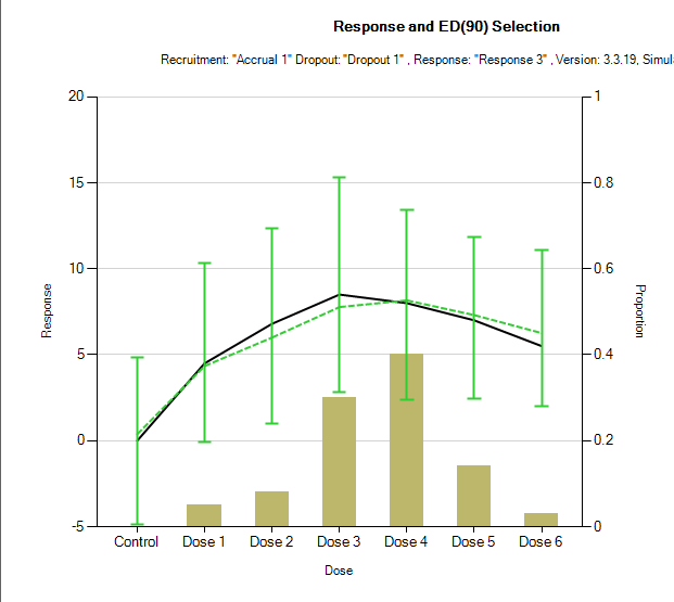
The additional term \(\zeta_d\) is a per dose ‘off-curve’ effect. It allows for a secondary non-parametric dose effect over and above the logistic model. It has been used in circumstances in which there is actually some falling away of effect at the highest dose. This is an example mean fit from 100 simulations. The model fit and error bars are in green, and the true dose responses are shown by the black line.
\(\zeta_d\) is modelled as:
\[\zeta_d \sim \text{N}(0, a_4^2)\]
conditioned that
\[\sum_{d}^{}\zeta_{d} = 0\]
And \(a_4^2\) has an inverse gamma prior:
\[a_{4}^{2}\sim IG\left( \frac{\Lambda_{n}}{2},\frac{\Lambda_{\mu}^{2}\Lambda_{n}}{2} \right)\]
The following independent prior distributions are assumed:
\[a_1\sim \text{N}(\Lambda_1, \lambda_1^2)\] \[a_2\sim \text{N}(\Lambda_2, \lambda_2^2)\] \[a_3\sim \text{N}^+(\Lambda_3, \lambda_3^2)\]
A typical recommended value for the center of the prior distribution of \(\alpha_4\) is the largest expected likely deviation in true response from the underlying logistic with a weight of 1. The effect of this prior is then checked through simulation of a range of plausible dose response profiles, with a range of designs to check the sensitivity of the final estimate of response to this prior. Additionally, see here for help with specifying an inverse gamma distribution with center and weight.
In this model, compared to the ‘plain’ 3-parameter logistic above, it is important that the true ED50 lies within the expected dose range, and that the prior for the ED50, \(a_3\), has the majority of its probability mass in the available dose range. For example, if the range of the effective dose strengths is from 0 to \(\nu_D\) then a typical ‘weakly informative’ prior for \(a_3\) would be:
\[a_{3}\sim N^{+}\left( \frac{\nu_{D}}{2},\left( \frac{\nu_{D}}{2} \right)^{2} \right)\]
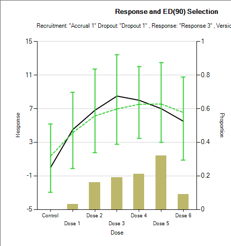
Using a weaker prior, such as \(\text{N}^+(\nu_D, \nu_D^2)\) leads to a more linear fit. With just this change to the prior for \(a_3\) the average of the estimated of the mean response changes from the graph above to:
Sigmoid Model
A sigmoid model (\(\text{E}_{\text{max}}\)) provides a coherent parameterization of the dose response trend similar to the 3-parameter logistic, but with one extra shape parameter, \(a_4\).
The model formula is:
\[\theta_{d} = a_{1} + \frac{(a_{2} - a_{1})v_{d}^{a_{4}}}{{a_{3}}^{a_{4}} + v_{d}^{a_{4}}}\]
The interpretation of the four parameters is:
- \(a_1\)
- the estimated dose response for a dose of strength 0
- \(a_2\)
- the estimated dose response for a dose of strength \(\infty\) (slight difference from Logistic models)
- \(a_3\)
- the estimated ED50, the dose that has 50% of the dose response maximum attainable effect (\(a_2-a_1\))
- \(a_4\)
- controls the slope of the dose response model at the ED50. A larger value of \(a_4\) corresponds to a steeper slope. A value of \(a_4=1\) makes the Sigmoid model equivalent to a Three Parameter Logistic model with \(a_2\) equal to \(a_1 + a_2\) from the Sigmoid model. A value of \(a_4\) approaching 0 corresponds to a dose response model that is nearly flat at \(\frac{a_{1} + a_{2}}{2}\). By differentiation, it can be seen that the slope where the effective dose \(\nu_d=a_3\) is \((a_{2} - a_{1})\frac{a_{4}}{4a_{3}}\).
The following independent prior distributions are assumed:
\[a_1\sim \text{N}(\Lambda_1, \lambda_1^2)\] \[a_2\sim \text{N}(\Lambda_2, \lambda_2^2)\] \[a_3\sim \text{N}^+(\Lambda_3, \lambda_3^2)\] \[a_3\sim \text{N}^+(\Lambda_4, \lambda_4^2)\]
The advantage of this model is that it is considerably more flexible than the logistic, but still more efficient to estimate than an NDLM. This model (if applicable) is ideal if the target is an Effective Dose (ED) such as an ED90. Estimating an ED requires estimating the response on control, the maximum response, and the gradient which is requires a lot of data to do well if using no model or a smoothing model such as one of the NDLMs. With the 4-parameter Sigmoid model (or 3-parameter logistic – but that has a more limited applicability due to being significantly less flexible in shape), it’s usually not an issue to estimate the EDx well.
The caveats to using this model are:
Whilst being much more flexible than the logistic, it still has model assumptions, in particular monotonicity, that must be met for this to be a reasonable model to be used.
The curve is only well estimated if the true ED50 lies within the doses tested.
Like the hierarchical logistic model above, the prior for \(a_3\) should be weakly informative, with the majority of its probability mass in the available dose range. So similarly, if the range of the effective dose strengths is from 0 to \(\nu_D\) then a typical ‘weakly informative’ prior for \(a_3\) would be: \[a_3 \sim N^{+}\left( \frac{\nu_{D}}{2},\left( \frac{\nu_{D}}{2} \right)^{2} \right)\]
U-Shaped Model
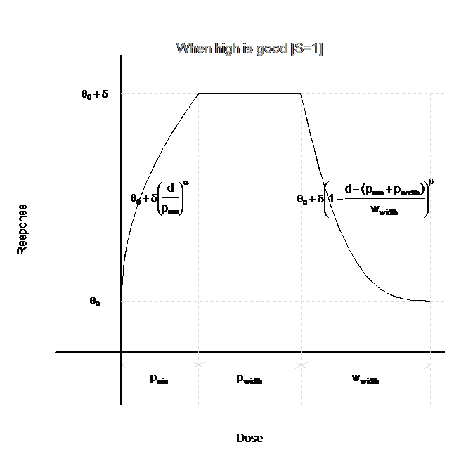
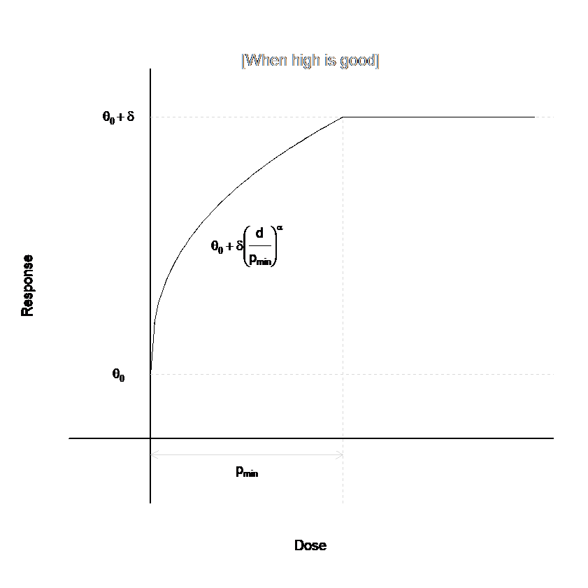
The U-shaped model when the allows for an initial increase (decrease) in the dose response with dose, followed by a leveling out of the mean, then a decrease (increase). Whether the U-Shaped model increases then decreases or decreases then increases is specified by the user on the Dose Response tab. An example curve for this model is given in the figure below.
The dose-response curve can be characterized in four different regions of doses. For the first region, which contains the lowest doses, \(0<\nu_d<p_{min}\), the dose-response curve is increasing (decreasing):
\[\theta_{d} = \theta_{0} + S \cdot \delta \cdot \left( \frac{\nu_{d}}{p_{\min}} \right)^{\alpha}\]
The next region is the plateau, where the dose-response curve is constant. For \(p_{min} < \nu_d < p_{min}+p_{width}\): \[\theta_d=\theta_0 + S\cdot\delta\] For the third region, the dose-response curve is decreasing (increasing). For \(p_{min}+p_{width} < \nu_d < p_{min}+p_{width} + w_{width}\),
\[\theta_{d} = \theta_{0} + S \cdot \delta \cdot \left( 1 - \frac{\nu_{d} - \left( p_{\min} + p_{width} \right)}{w_{width}} \right)^{\beta}\]
For the final region, the dose-response curve is again constant, at the same level as the zero-dose. For \(\nu_d > p_{min}+p_{width} + w_{width}\), \[\theta_d = \theta_0\]
The parameters of the model are described below:
\(S\) is \(1\) or \(-1\), as determined by the Model is increasing/decreasing radio buttons. \(S=1\) if Model is Increasing is selected, indicating that the model starts increasing at low doses.
\(\theta_0\) represents the zero-strength dose response. Its prior is: \[\theta_0 \sim \text{N}(\mu_0, \sigma_0^2)\]
\(\delta\) represents the maximal change in response from the zero-strength dose. It is restricted to be positive, and has a prior of: \[\delta \sim \text{N}^+(\mu_\delta, \sigma_\delta^2)\]
\(p_{min}\) represents the lowest dose at which the maximal change in response from the zero-strength is achieved. It is restricted to be positive, and has a prior of: \[p_{min} \sim \text{N}^+(\mu_{min}, \sigma_{min}^2)\]
\(p_{width}\) represents the width of the plateau – the region where all doses achieve maximal change in response from the zero-strength dose. It is restricted to be positive, and has a prior of: \[p_{width} ~ \sim \text{N}^+(\mu_{width}, \sigma_{width}^2)\]
\(w_{width}\) represents the width of the region for doses beyond the plateau, where response is returning to the zero-strength dose level. It is restricted to be positive, and has a prior of: \[w_{width} ~ \sim \text{N}^+(\mu_{w}, \sigma_{w}^2)\]
\(\alpha\) determines the rate of change of the dose response curve for doses below the plateau. Values less than \(1\) indicate a rapid initial change from baseline, with slower change as the plateau is reached. Values greater than \(1\) indicate a slow initial change from baseline, with more rapid change as the plateau is reached. To help avoid identifiability issues, \(\alpha\) is restricted to be between \(10^{-1}\) and \(10^{1}\). \(\alpha\)’s prior is: \[\alpha \sim \text{LN}^*(\mu_\alpha, \sigma_\alpha^2)\] where \(\text{LN}^*()\) represents the lognormal distribution with truncation constraints at \(10^{-1}\) and \(10^{1}\).
\(\beta\) determines the rate of change of the dose response curve for doses beyond the plateau. Values less than \(1\) indicate a slow initial change from the plateau level, with more rapid change subsequently. Values greater than \(1\) indicate a rapid initial change from the plateau level, with slower change subsequently. To help avoid identifiability issues, \(\beta\) is restricted to be between \(10^{-1}\) and \(10^{1}\). The prior on \(\beta\) is: \[\beta \sim \text{LN}^*(\mu_\beta, \sigma_\beta^2)\]
The U-shaped model has seven free parameters, and thus it is inadvisable to use such a model for dose-finding trial designs that contain only a few dose levels. When a small number of doses are available, it may help to constrain the values of \(\alpha\) and \(\beta\) by utilizing small standard deviations in the priors.
Plateau Model
The plateau model is a special case of the U-shaped model, in which \(p_{width}=\infty\). That is, there is no return to baseline for high doses. This model eliminates three parameters from the U-Shaped model, since \(p_{width}\), \(w_{width}\), and \(\beta\) are not used. See the figure below to see an example dose response model for the plateau model that mimics the beginning of the U-Shaped model above.
3 Parameter Exponential Logistic (Dichotomous Only)
The 3-parameter exponential logistic model has the following structure:
\[\theta_d = a_1 + a_2 \nu_d^{a_3}\]
Where \(\nu_d\) is the effective dose strength of dose \(d\). This is a logistic model for the dichotomous endpoint because \(\theta_d\) is the log odds ratio of the probability of the response, \(P_d\) at dose \(d\).
The exponent parameter \(\alpha_3\) allows the change in slope at the lower end of the curve to be asymmetric in comparison to the change in curve at the upper end of the curve.
The priors for the parameters are:
\[a_1\sim \text{N}(\Lambda_1, \lambda_1^2)\] \[a_2\sim \text{N}(\Lambda_2, \lambda_2^2)\] \[a_3\sim \text{N}^+(\Lambda_3, \lambda_3^2)\] The interpretations of the parameters defining this model are:
- \(a_1\)
- the dose response for a dose with strength 0
- \(a_2\)
- the slope associated with the exponentiated dose strength
- \(a_3\)
- a shape parameter modifying the effective dose strength through exponentiation.
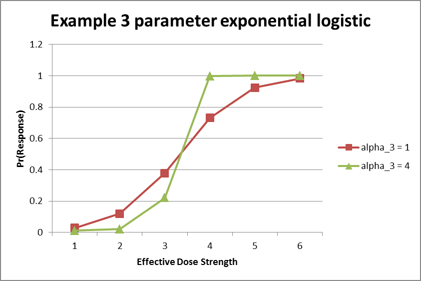
The figure below shows an example of two different 3-parameter exponential logistic model fits. Notably, the fit shown in green has an \(a_3\) parameter greater than \(1\), which leads to faster increases of the response rate model as the effective dose strength increases.
Hierarchical Model
Like the Independent Dose Model, the hierarchical model treats the arms as if they are an unordered set of treatments, but unlike the Independent Dose Model the Hierarchical Model shares information between doses included in the model. The hierarchical model is a way of encouraging the estimates of arm responses to be similar, and the degree of this encouragement can be controlled using parameters of the prior distribution. The hierarchical model assumes that the arm parameters are drawn from the same normal distribution:
\[\theta_d \sim \text{N}(\mu, \tau^2)\]
Where \(d\) is the set of doses included in the model. The prior distributions for \(\mu\) and \(\tau^2\) are
\(\mu \sim \text{N}(\Lambda_\mu, \lambda_\mu^2)\)
and
\[\tau^{2}\sim \text{IG}\left(\frac{\tau_{n}}{2},\frac{\tau_{\mu}^{2}\tau_{n}}{2} \right)\]
where \(\tau_\mu\) is a central value for \(\tau\), and \(\tau_n\) is the prior weight. \(\tau^2\) governs the amount of information shared between doses in the model. The estimates of the dose parameters can be encouraged to be close together by choosing a small value for \(\tau_\mu\) and a large value for \(\tau_n\). See here for a tool to help understand the inverse gamma distribution specified by center and weight parameters.
The control arm can be included in the hierarchical model if it is desired to encourage the experimental arms to be similar to the control arm, or excluded from it if the experimental arms are encouraged to be similar to each other but not necessarily to the control arm. This is not true with time-to-event data, when the control arm can only be excluded from the hierarchical model.
Linear Model
The linear model uses a strong assumption of exact linearity between the responses and the dose strengths. (For dichotomous models, the linearity is on the log-odds scale, and the linearity is on the log hazard ratio scale for TTE models.) The model is
\[\theta_d=\alpha+\beta\nu_d\] for all doses \(d\) in the model. Both \(\alpha\) and \(\beta\) are given normal prior distributions:
\[\alpha \sim \text{N}(\Lambda_\alpha, \lambda_\alpha^2)\] \[\beta \sim \text{N}(\Lambda_\beta, \lambda_\beta^2)\]
The linear model is appropriate when there is strong scientific knowledge that the shape of the response curve should be linear as a function of dose strength. Note that if an arm has a dose strength between two other arms in the model, its response will always be estimated to be between the responses of those two arms. As a result, the linear model may not be appropriate in combination with certain decision quantities such as Pr(Max), because some doses are guaranteed to have probability zero of being the best arm. If the control arm is included in the linear model and it has the smallest dose value, then all experimental arms will always have exactly the same probability of being better than control.
We recommend creating scenarios where the true parameters deviate from linearity and simulating them to test the robustness of a design based on the linear model.
For dichotomous models, the linear model replaces the 2-parameter logistic model available in FACTS versions before 6.4. The two models are identical.
Hierarchical Linear Model
A more flexible version of the linear model is the hierarchical linear model. This model encourages the arm responses to have a linear-like shape, but also includes a term allowing parameters to deviate from linearity when appropriate. The arm parameters satisfy the relationship
\[\theta_d = \alpha + \beta \nu_d + \zeta_d\] where the \(\alpha\) and \(\beta\) parameters are as in the linear model, with prior distributions
\[\alpha \sim \text{N}(\Lambda_\alpha, \lambda_\alpha^2)\] \[\beta \sim \text{N}(\Lambda_\beta, \lambda_\beta^2)\] and the \(\zeta_d\) parameters are the deviations from linearity. These deviations are assumed to have a normal distribution constrained so that their average value is zero:
\[\zeta_d \sim \text{N}(0, \tau^2) \text{ with } \sum_d\zeta_d=0.\]
The prior distribution for \(\tau^2\) is
\[\tau^{2}\sim\text{IG}\left(\frac{\tau_{n}}{2},\frac{\tau_{\mu}^{2}\tau_{n}}{2} \right)\]
If \(\tau^2\) is small, which can be encouraged by choosing \(\tau_\mu\) to be small and \(\tau_n\) to be large, then the dose parameter estimates will lie close to a line. See here for help understanding FACTS’s parameterization of the inverse gamma distribution.
The hierarchical linear model is a good choice when, for example, one expects a linear relationship between the dose strengths and the response but one is not prepared to assume exact linearity. It can also be a good way of encouraging, but not requiring, monotonicity in the response.
2D Treatment Dose Response Models
If on the Study > Treatment Arms tab, the “Use 2D treatment arm model” option has been checked, the user may either use any of the 1D Dose Response options described above, or may use a dose response model specifically modelling the two dosing dimensions.
If using one of the 1D dose response models, the effective dose strength \(\nu_d\) is as specified by the user on the “Select doses to be used in the trial” tab. These calculated dose levels are forced to be distinct values, and this results in a 1D ordering of the combinations.
There are also three 2D Dose Response models that can be used:
2D Continuous Factorial Model
2D Discrete Factorial model
2D NDLM
These are described in the next sections.
The 2D dose response models work with a slightly different notation to accommodate that treatments are defined as the combination of two factors. Rather than \(\theta_i\) being the estimated mean of the dose response estimate for dose \(i\), the estimated dose response for the treatment created from row factor level \(r\) and column factor level \(c\) is denoted \(\theta_{rc}\). \(Y_{rc}\) denotes the mean of the observed data in the cell.
In the continuous case, the likelihood for the data is,
\[Y_{rc} \sim \text{N}(\theta_{rc}, \sigma^2)\] \[\sigma^{2}\sim\text{IG}\left(\frac{\sigma_{n}}{2},\frac{\sigma_{\mu}^{2}\sigma_{n}}{2} \right)\]
Where the form of \(\theta_{rc}\) varies based on dose response model selection.
Similarly, in the dichotomous case,
\[Y_{rc} \sim \text{Bernoulli}(P_{rc})\] \[P_{rc} = \frac{e^{\theta_{rc}}}{1 + e^{\theta_{rc}}}\]
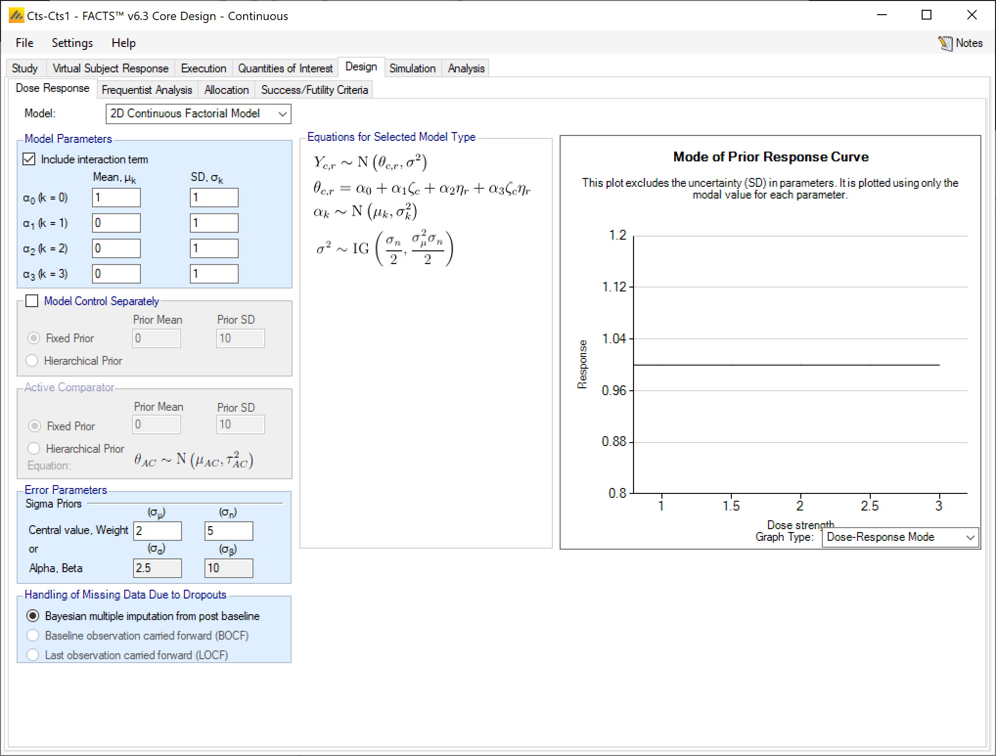
2D Continuous Factorial Model
The 2D Continuous Factorial Model fits a regression on the dose response that uses the numeric dose strength as a continuous valued covariate. The dose response (with \(\eta_r\) and \(\zeta_c\) denoting dose strength of the row level and column level, respectively) is modeled as:
\[\theta_{rc} = \alpha_0 + \alpha_1 \zeta_c + \alpha_2 \eta_r + \alpha_3\zeta_c \eta_r\] With priors
\[\alpha_0 \sim \text{N}(\mu_0, \sigma_0^2)\] \[\alpha_1 \sim \text{N}(\mu_1, \sigma_1^2)\] \[\alpha_2 \sim \text{N}(\mu_2, \sigma_2^2)\] \[\alpha_3 \sim \text{N}(\mu_3, \sigma_3^2)\]
Then, \(\alpha_0\) is the response at the control combination, \(\alpha_1\) is the linear coefficient of the response to the column factor strengths \(\zeta_c\), and \(\alpha_2\) is the linear coefficient of the response to the row factor strengths \(\eta_r\).
The user has the option to simplify the model and exclude the interaction term \(\alpha_3\), which is the coefficient of the product of the two factor strengths.
Note that despite being called “continuous” this dose response model applies to all endpoints. It’s called continuous because the coefficients act on the dose strengths as continuous measures of strength.
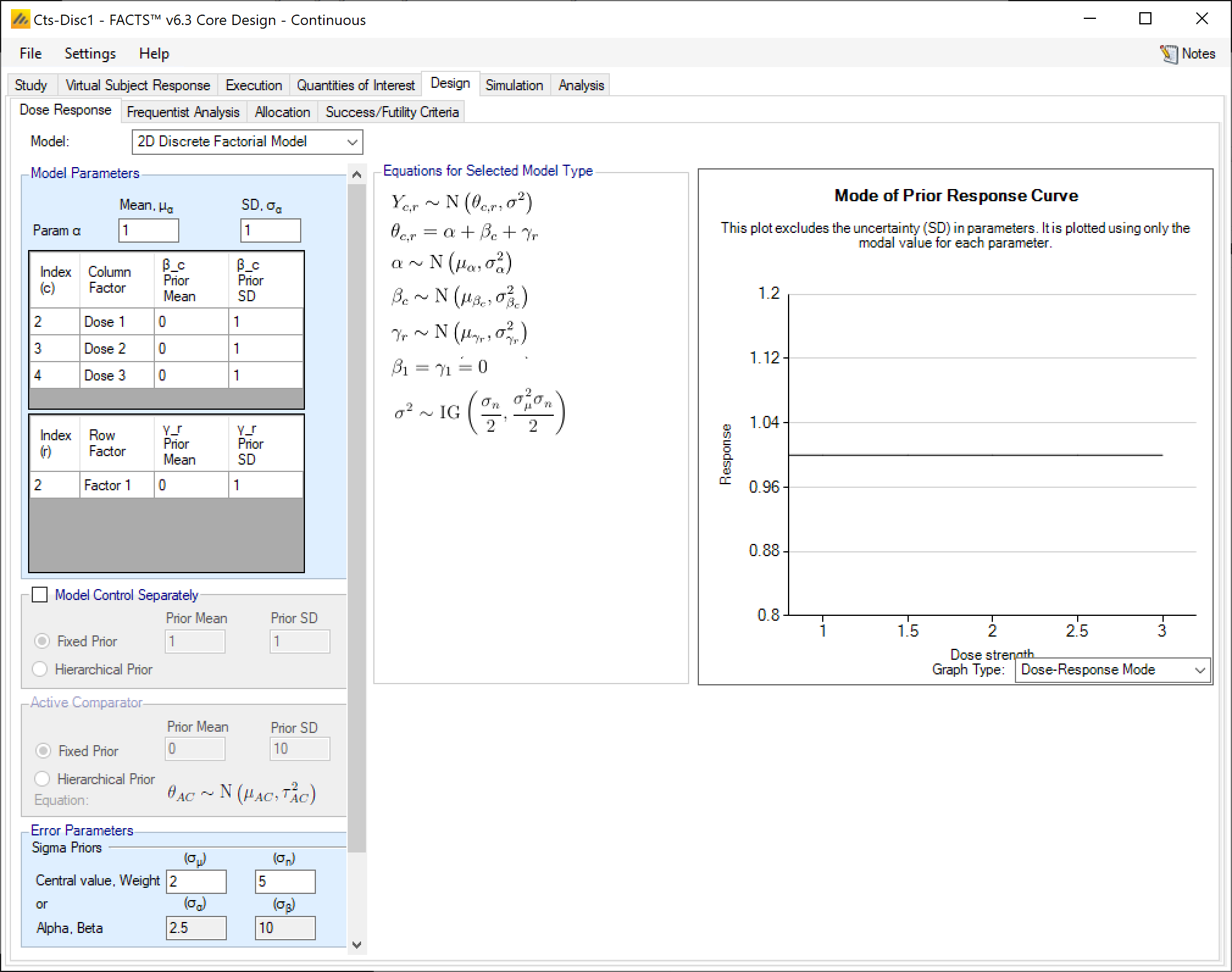
2D Discrete Factorial Model
The 2D Discrete Factorial Model fits a regression on the dose response that uses the dose strength as a factor covariate rather than a numeric dose strength. Each dose is an independent level within each row or column factor, so any dose is equidistant from all other doses
\[\theta_{rc} = \alpha + \gamma_r + \beta_c\]
With priors
\[\alpha \sim \text{N}(\mu_\alpha, \sigma_\alpha^2)\]
\[\beta_c \sim \text{N}(\mu_{\beta_c}, \sigma_{\beta_c}^2)\] \[\gamma_r \sim \text{N}(\mu_{\gamma_r}, \sigma_{\gamma_r}^2)\]
The parameters associated with lowest level of each factor, \(\gamma_0\) and \(\beta_0\), are constrained to be \(0\).
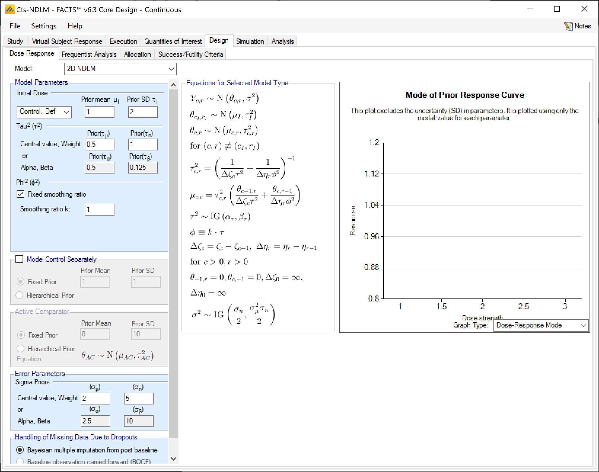
2D NDLM
The 2-D NDLM Model takes the idea of smoothing across doses that was used in the standard NDLM model, but smooths across row factors and column factors separately.
The Base Model, with Control Included
The treatment effect for the combination of level \(r\) in the row factor and level \(c\) in the column factor is denoted as \(\theta_{rc}\), and \(Y_{rc}\) is the observed data in that cell. The borrowing parameters are denoted as \(\phi\) for the row factor smoothing, and \(\tau\) for the column factor smoothing. The dose strengths are denoted as \(\nu_r\) for the row factors, and \(\omega_c\) for the column factors. Let \(\Delta \nu_r = \nu_r - \nu_{r-1}\) and \(\Delta \omega_c = \omega_c - \omega_{c-1}\) (for \(r>0\) and \(c>0\)). For notational convenience at the grid edge, let \(\theta_{-1, c} = 0\), \(\theta_{r,-1}\), \(\Delta\nu_0\equiv\infty\), and \(\Delta\omega_0\equiv\infty\).
The 2-D NDLM Model with control included in the model can then be specified as:
\[\theta_{0,0} \sim \text{N}(\mu_0, \tau_0^2)\] \[\theta_{rc} \sim \text{N}(\mu_{rc}, \tau_{rc}^2)\] where
\[\tau_{rc}^{2} = \left( \frac{1}{\mathrm{\Delta}\nu_{r}\phi^{2}} + \frac{1}{\mathrm{\Delta}\omega_{c}\tau^{2}} \right)^{- 1}\]
\[\mu_{rc} = \tau_{rc}^{2}\left( \frac{\theta_{r - 1,c}}{\mathrm{\Delta}\nu_{r}\phi^{2}} + \frac{\theta_{r,c - 1}}{\mathrm{\Delta}\omega_{c}\tau^{2}} \right)\]
with priors
\[\tau^{2}\sim\text{IG}\left( \frac{\tau_{n}}{2},\frac{\tau_{\mu}^{2}\tau_{n}}{2} \right)\]
\[\phi^{2}\sim\text{IG}\left( \frac{\phi_{n}}{2},\frac{\phi_{\mu}^{2}\phi_{n}}{2} \right)\]
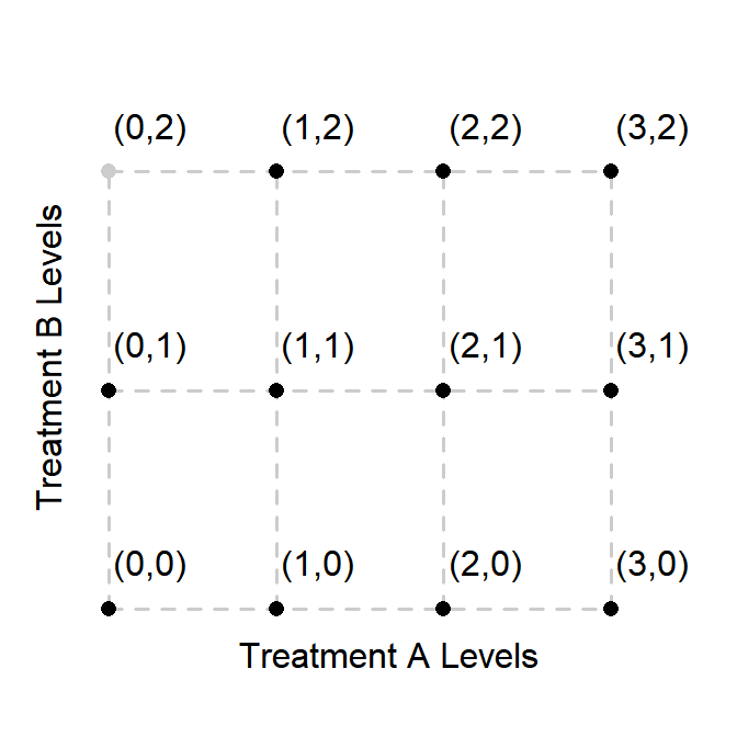
Note: that not all combinations of \(r\) and \(c\) will have data associated with them. However, FACTS will still evaluate the prior at all combinations. Thus, in the situation depicted below where the grayed-out point indicates a treatment combination with no allocation, \(\theta_{1,2}\) is not modeled conditioned only on \(\theta_{1,1}\). \(\theta_{0,1}\) also informs on \(\theta_{1,2}\) via \(\theta_{0,2}\).
Fix smoothing ratio for row factor and column factor
Optionally, the user might want to specify the row factor borrowing as a function of the column factor borrowing:
\[\phi\equiv k \cdot \tau\] where \(k\) is a user-specified constant. This can be performed by selecting “Fixed smoothing ratio” in the \(\phi^2\) prior specification area.
Control not in model, no zero-level doses
If neither treatment arm allows zero-level doses (e.g. like one would expect if the column factor represented doses and the row factor represented frequency), then a prior for the lowest dose would instead be needed as input from the GUI:
\[\theta_{1,1} \sim \text{N}(\mu_1, \tau_1^2)\]
Baseline Adjusted Dose Response Models (Continuous Only)
If a baseline endpoint is simulated, the user has the option of adding a linear covariate effect to the dose response model. If the chosen dose response model states that for dose \(d\), \[Y\sim \text{N}(\theta_d, \sigma^2)\] then the distribution including the baseline adjustment term is \[Y\sim \text{N}(\theta_d+\beta Z, \sigma^2)\] where \(Z\) is the standardized baseline value \(\left(Z=\frac{X-\bar X}{s_x}\right)\), and \(\beta\) is an estimated parameter that is distinct from any parameter called \(\beta\) within the dose response model.
The baseline adjustment model uses a normal prior for \(\beta\) for which the user enters a mean and standard deviation.
The VSR based simulation of baseline is more general than the model adjustment for baseline (this is to allow baseline to be incorporated in a number of different ways). This means that the parameters entered in the VSR (for example the \(\beta\) parameter) will not always match the corresponding parameter estimated in the dose response model.
As a simple example, suppose we enter into the VSR response \(Y\sim \text{N}(\mu_Y, \sigma_Y^2)\), baseline \(X\sim \text{N}(\mu_X, \sigma_X^2)\), and use the baseline adjustment (\(c\), \(s\), and \(\beta_{VSR}\) are user inputs) so the actual simulated response \(Y\) is \(Y^{'} = Y + \beta_{VSR}\frac{X - c}{s}\).
If the values of \(c\) and \(s\) used in the baseline adjustment are the same as the mean \(\mu_X\) and standard deviation \(\sigma_X\) of the simulated baseline, then the \(\beta_{VSR}\) will converge to the estimated \(\beta\) parameter as the sample size of the study increases. If \(c\ne\mu_X\) or \(s\ne\sigma_X\), then the estimated \(\beta\) will not converge to the \(\beta_{VSR}\) used in data simulation. Additionally, if the baseline values are simulated from a truncated normal distribution, then the estimated \(\beta\) will not converge to \(\beta_{VSR}\).
Control and Comparator Priors
For most All continuous and dichotomous models except the U-shaped and Plateau models. dose response models the control arm can be modeled either as part of the dose response model or separately. If it is modeled separately, it may have a simple user specified Normal prior or a “historical” prior. A historical prior in FACTS is a hierarchical prior that models the response on control as coming from a distribution that also contains trial outcomes from external historical studies.
The active comparator is always modeled separately, and as with a control arm modeled separately, it can be modeled with a user specified Normal prior or a “historical” prior.
When a user specified Normal prior is used, the user specifies the mean and standard deviation of the prior normal distribution for \(\theta_0\). This is useful if the control response is not thought to be consistent with the model being used to model the study doses – for instance if using an NDLM and there might be a sharp step in response from control to the lowest dose.
If “Hierarchical Prior” is selected for either the control arm or an Active Comparator arm, a “Hierarchical Priors” tab is created.
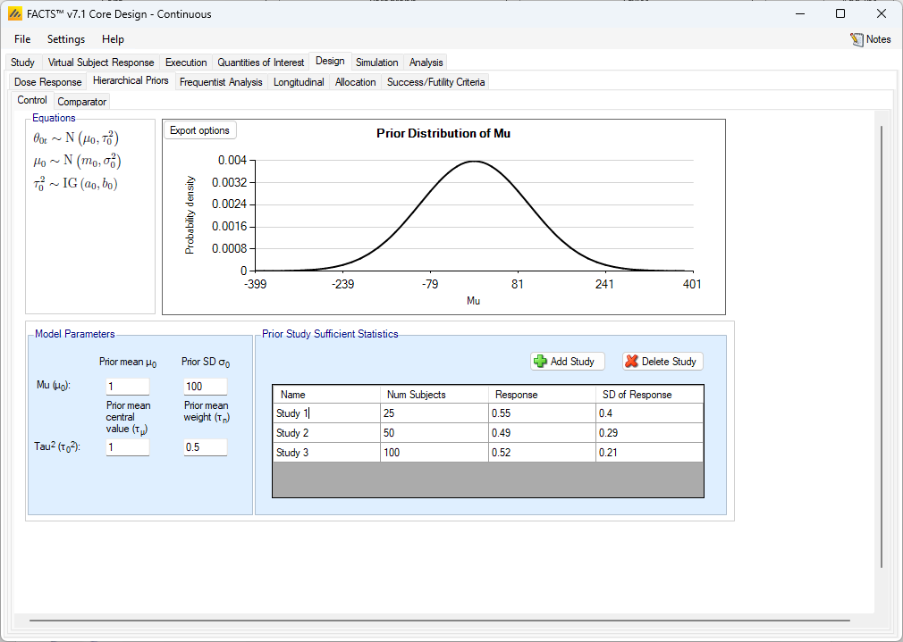
Hierarchical Priors
If a hierarchical prior is used for either the Control or Active Comparator arm, then FACTS will estimate a prior for that arm using external data that the user provides. This prior is estimated through a hierarchical model, and then the in-study data collected on subjects randomized to that arm are used to estimate the posterior distribution for the arm.
To specify a hierarchical prior, the user specifies the sufficient statistics from each historical study. These are:
Continuous: the mean response and the SD of the response of the control or active comparator arm and the number of subjects observed.
Dichotomous: the observed number of responders and the number of subjects observed in the study.
Time-to-Event: the number of events and the amount of exposure within each bin in the piecewise model.
The information from the historical studies can be ‘down-weighted’ by decreasing the effective information in the sample size. For continuous, this can be done by decreasing the sample size by a percentage. For dichotomous, both the number of responders and the number of subjects would be decreased by a percentage. For time-to-event, multiplying the number of events and the exposure by the same fraction will reduce the information in the study without changing the reported hazard rate.
The hierarchical models for the control or active comparator rates are very similar across the endpoints. They are briefly described below.
The model used for incorporating data from previous trials is as follows:
\[\theta_{0t} \sim \text{N}(\mu_0, \tau_0^2) \text{ for } \tau=0,1,2,\ldots,T\] where \(\theta_{0t}\) is the mean for the control arm in trial \(t\) (\(t=0\) for the current trial and \(t=1,2,\ldots,T\) for previous trials). A user needs to specify appropriate priors for the hyper-parameters:
\[\mu_0 \sim \text{N}(m_0, \sigma_0^2)\] \[\tau_0^2 \sim \text{IG}(a_0, b_0)\]
The model used for incorporating data from previous trials is as follows:
\[\theta_{0t} \sim \text{N}(\mu_0, \tau_0^2) \text{ for } \tau=0,1,2,\ldots,T\] where \(\theta_{0t}\) is the log-odds for the control arm in trial \(t\) (\(t=0\) for the current trial; \(t=1,2,\ldots,T\) for previous trials). A user needs to specify appropriate priors for the hyper-parameters:
\[\mu_0 \sim \text{N}(m_0, \sigma_0^2)\] \[\tau_0^2 \sim \text{IG}(a_0, b_0)\]
The prior distributions for the hyper-parameters of the hierarchical model. The hyper-parameters are the mean and standard deviation of Normal distribution for the log hazard ratios of the event rates of the historical studies and the current study.
The model used for incorporating data from previous trials is as follows:
\[\lambda_{st}=\lambda_s \exp(\gamma_t) \text{ for } t=0,1,2,\ldots,T\] where \(\lambda_{st}\) is the hazard rate for the control arm in segment \(s\) (\(s=1,2,\ldots,S\)) for previous trial \(t\) (\(t=1,2,\ldots,T\)) and \(\lambda_{s0}\) is the hazard rate for the current control arm in segment \(s\); \(\lambda_s\) is a base hazard for segment \(s\); and \(\gamma_t\) is the log hazard ratio between that base rate and the \(\lambda_{st}\) values.
The following hierarchical model is used
\[\gamma_t \sim \text{N}(\mu_\gamma, \tau_\gamma^2) \text{ for } t=0,1,2,\ldots,T\] Users specify priors for the hyper-parameters:
\[\mu_\gamma \sim \text{N}(m_\gamma, t_\gamma^2)\] \[\tau^2 \sim \text{IG}(a_\gamma, b_\gamma)\]
The formulation above is not identifiable as changes in \(\lambda_s\) can be compensated for by changes in the \(\gamma_t\) values (thus, one can use different combination of \(\lambda_s\) and \(\gamma_t\), but acquire the same set of values \(\lambda_{st}\) and thus the same likelihood). To avoid this difficulty, we use the above formulation but fix \(\gamma_0 = 0\). In addition to preserving the identifiability of the structure, this constraint allows \(\lambda_s\) to have the interpretation of being the hazard rate for the current control arm, and thus the prior on \(\lambda_s\) from the main dose response may be used as the prior for \(\lambda_s\).
Setting Priors for Hierarchical Model Hyper Parameters
Unless the intent is to add information that is not included in the historic studies, the hyper parameters can and should be set so that they are ‘weak’ priors, centered on the expected values.
In this case the following would be reasonable:
Set the prior mean value for Mu as the mean of the mean responses on the control arm in the historic studies
Set the prior SD for Mu equal to the average SD of response divided by the square root of the number of studies.
Set the center for tau to the same value as the prior SD for Mu.
Set the weight for tau to be < 1.
One can traverse the spectrum from ‘complete pooling of data’ to ‘completely separate analyses’ through the prior for tau. If the weight of the prior for tau is small (relative to the number of studies), then (unless set to a very extreme value) the mean of the prior for tau will have little impact and the degree of borrowing will depend on the observed data.
To give some prior preference towards pooling or separate analysis the weight for tau has to be large (relative to the number of historic studies) – to have a design that is like pooling all the historic studies the mean for tau needs to be small (say 10% or less of the value suggested above). For there to be no borrowing from the historic studies the value for tau needs to be large (say 10x or more the value suggested above).
The best way to understand the impact of the priors is try different values and run simulations.
Bayesian Augmented Control (BAC) Example:
It is easiest to study the impact of BAC in a simplified version of the trial being designed, for example use a 2 arm fixed design with ‘no model’, no adaptation, no longitudinal modeling, etc.
For instance, in a continuous setting with an expected sample size of 50 on control, a mean response of 5 and an SD in the response of 2, looking at the effect of having 4 prior, similarly sized studies:
| Number of subjects | Mean Response | SD of Response | |
|---|---|---|---|
| Study 1 | 50 | 4.76 | 2 |
| Study 2 | 50 | 4.93 | 2 |
| Study 3 | 50 | 5.07 | 2 |
| Study 4 | 50 | 5.24 | 2 |
For simplicity we have just varied the means of the studies – they are all consistent with a normally distributed estimate, with mean of 5 and a standard error of \(\frac{2}{\sqrt{50}}\).
By simulating a fixed trial with a sample size of 100 and fixed 1:1 allocation between control and a study arm we can easily observe the effects of a BAC on the control arm. Creating 6 VSR profiles with sigma = 2, and the same mean response for control and the study arm in each profile of: 4.53, 4.76, 5.07, 5.24 and 5.47 we can look at the bias of the final estimate and the shrinkage in the SD of the estimate that could be brought about by using BAC:
| True Mean | Raw mean | Raw SD | Estimate inc BAC | SD inc BAC | Bias | Effective additional Subjects |
|---|---|---|---|---|---|---|
| 4.53 | 4.55 | 0.28 | 4.64 | 0.255 | 2.1% | 11.1 |
| 4.76 | 4.78 | 0.28 | 4.83 | 0.250 | 1.0% | 13.5 |
| 4.93 | 4.95 | 0.28 | 4.96 | 0.248 | 0.2% | 14.3 |
| 5.07 | 5.09 | 0.28 | 5.07 | 0.248 | -0.4% | 14.2 |
| 5.24 | 5.26 | 0.28 | 5.20 | 0.250 | -1.1% | 13.2 |
| 5.46 | 5.49 | 0.28 | 5.38 | 0.255 | -1.9% | 10.7 |
Note it is important to use the column “SD Mean resp 1” from the simulations file to see the SD of the estimate and not use the SD of the estimates in the summary table.
The small shrinkage in the SD is more impressive when viewed in terms of how many additional subjects would have to be recruited to achieve the same shrinkage in the raw estimate. These are useful savings for small additional bias.
The “effective additional subjects” was calculated: \[\left( \frac{\text{True sigma}}{\text{AVG(SD Mean resp)}} \right)^{2} - \left( \frac{\text{True sigma}}{\text{AVG(SE Mean Raw Response)}} \right)^{2}\] where in this example \(\text{True sigma}\) was 2.
Inverse-gamma priors
FACTS uses inverse-gamma priors for parameters of variance – these are conjugate and allow efficient computation and avoid problems of convergence. Andrew Gelman’s 2006 paper however notes a potential problem with this model, the problem is specifically
When updating the estimate of the variance of a hierarchical model parameter there will be typically relative few actual data observations (e.g. relatively few historic studies for estimating the variance of the hyper parameter in a Bayesian Augmented Control model for the response on a control arm, and relatively few observations of the change in response from one dose to the next when using an NDLM dose-response model).
The conventional ‘non-informative’ gamma-prior of IG(0.001, 0.001) has an effect when the observed variance is small, of over-shrinking the posterior estimate of variance.
In FACTS this possibility arises in the dose response models in the context of priors for the \(\tau\) parameter for the NDLM models and the \(a_4\) parameter for the hierarchical logistic dose response model, where the number of observations is the number of doses or dose intervals.
To avoid the problem reported by Gelman we recommend using a weakly informative prior. Using the settings that control how the inverse-gamma distribution is parameterized (Settings > Options > Gamma Distribution Parameters), use the ‘center and weight’ options and use a weight of 1, with a ‘reasonable’ expectation for the upper limit difference in the values being modeled entered as the center for the SD. The inverse gamma distribution is the prior of the variance, so the center parameter being specified is more correctly an expectation of the square root of the mean of the variance.
We have created a tool that can help visualize the inverse gamma distribution and relate the center/weight parameterization, which FACTS uses by default, to the alpha/beta parameterization that is common.
This ‘reasonable’ upper limit for the difference is a value that a clinical team will usually have an intuition about: for the largest change in mean response from one dose to another for instance, it is (often)[## “If the trial has doses that are more closely spaced than usual, a smaller figure can be used.”] reasonable to assume that the upper limit for the expected change in response from one dose to the next is the ‘expected difference in effect size’ that might have been used to power the trial in a conventional setting.
In the dose response setting the smoothing parameters like \(\tau\) in the NDLM are nuisance parameters in the sense that they are necessary to estimate in order to get appropriate estimates of the dose response values, but are rarely of inferential interest on their own. This can ease some of the undue burden of setting a prior on \(\tau\). If it gives estimates of the dose responses that look like you expect This is subjective. The Per Sim: Response and Subject Alloc plot in FACTS can help assess this fit. , then it is generally good enough.
Handling Missing Data
FACTS allows a “pre-processing” step before fitting the dose response model that helps with handling of data that is missing due to dropouts. If a subject has incomplete data due to a dropout, the user may specify all dropouts have their unknown final endpoint treated as known with the following options:
BOCF (continuous only, requires baseline be simulated) – All dropouts are assumed to have a final endpoint equal to their observed baseline value.
LOCF (continuous or dichotomous, requires longitudinal data be present) – All dropouts are assumed to have a final endpoint equal to their last observed visit value. If no post-baseline visits are available, but the subject has a baseline visit value, then the baseline values is carried forward to their final endpoint.
Missing is failure (dichotomous only) – All dropouts are assumed to be failures (which may be coded as 0 or 1 depending on whether a response is considered a success).
Subjects who are imputed in this pre-processing step have final endpoint values known and used for the purposes of estimating the dose response curve. However, these pre-processed final endpoint values are not used in the updating on the longitudinal model, which is based only on observed visit data.
If the user does not specify one of the dropout imputation methods specified above, the dropout subjects and incomplete subjects (subjects who have not reached their final endpoint but are still continuing in the study) will have their final endpoints multiply imputed using Bayesian Multiple Imputation, described in the Longitudinal Modeling section.
Generally, patients with “no data” do not affect the posterior distribution, and thus are omitted from the analysis. However, one must take into account a subject can have no visit data but still have “data” based on these dropout imputation methods. For example, if one selects “missing as failure” and a patient drops out before any visit data is recorded, then the subject still supplies information through the dropout imputation (similarly for BOCF). However, if LOCF is selected and no visit data is available, there remains no information on the subject to be used for the LOCF dropout imputation, and thus these subjects are omitted from the analysis. All subjects are included if they either 1) have some visit data available, or 2) are dropouts before visit 1 with sufficient information to impute their final endpoint with this pre-processing step.
Time-to-Event Missingness
For a time-to-event endpoint, as is the convention in this endpoint, subjects are observed up to the time they have an event (or the end of follow up), so no subject drops out after having had an event. Subjects that do drop-out are included in the analysis as not having had an event up to the last observation of the subject.