In FACTS Core with a continuous endpoint there are 2 different ways to specify the virtual subject response:

Explicit specification of the continuous endpoint
Importation of an externally generated set of simulated subject results.

Explicitly Defined Continuous Response

Explicitly defined VSRs are the most common type specified in FACTS. In continuous endpoint designs, an explicitly defined VSR is specified by providing a mean response and patient level standard deviation of the response for each arm in the trial. In certain cases, based on the selections made in the Study Info tab, baseline VSRs and Longitudinal VSRs may also need to be specified.

Dose Response

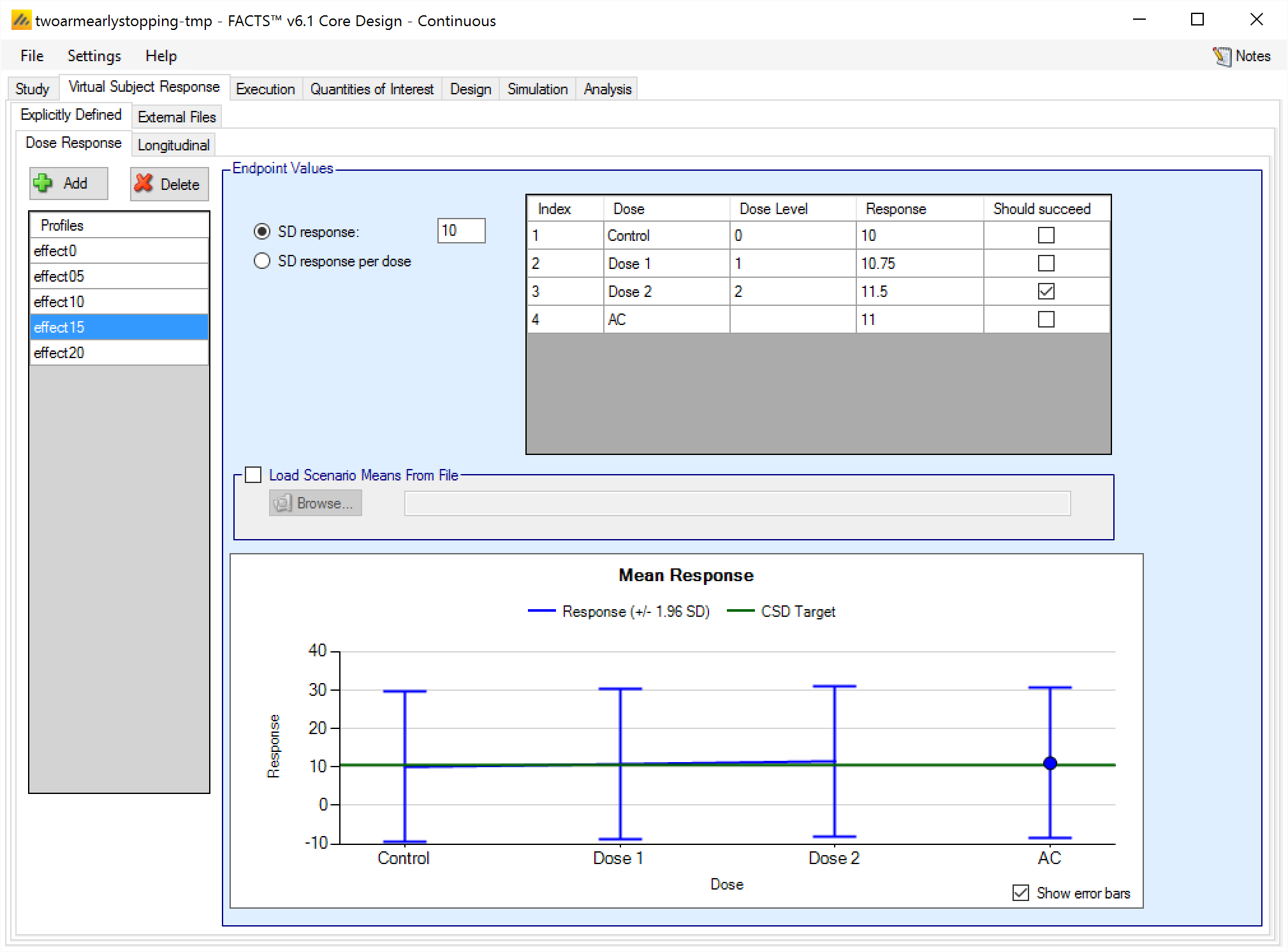
Dose response profiles can be added and deleted, and for each profile the user specifies:

The mean response for each treatment arm. If baseline is being simulated the user can select (on the Study tab) whether the response to be analyzed is the change from baseline or absolute response The mean response to be analyzed is always as specified on this tab, if the analysis is on change from baseline then the response specified here is change from baseline, if the response to be analyzed is absolute, then the response specified here is the absolute final score. , and depending on that selection the response specified on this tab is either change from baseline or absolute response.
The standard deviation of the response – either through a common SD of response for all treatment arms, or by specifying the standard deviation for the response on each treatment arm separately.
A check box that allows the user to specify whether a specific arm “should succeed” in that scenario.FACTS uses this value to report on the proportion of simulations that were successful and selected a ‘good’ treatment arm. The check box values do not effect the simulation code, just how output is reported.

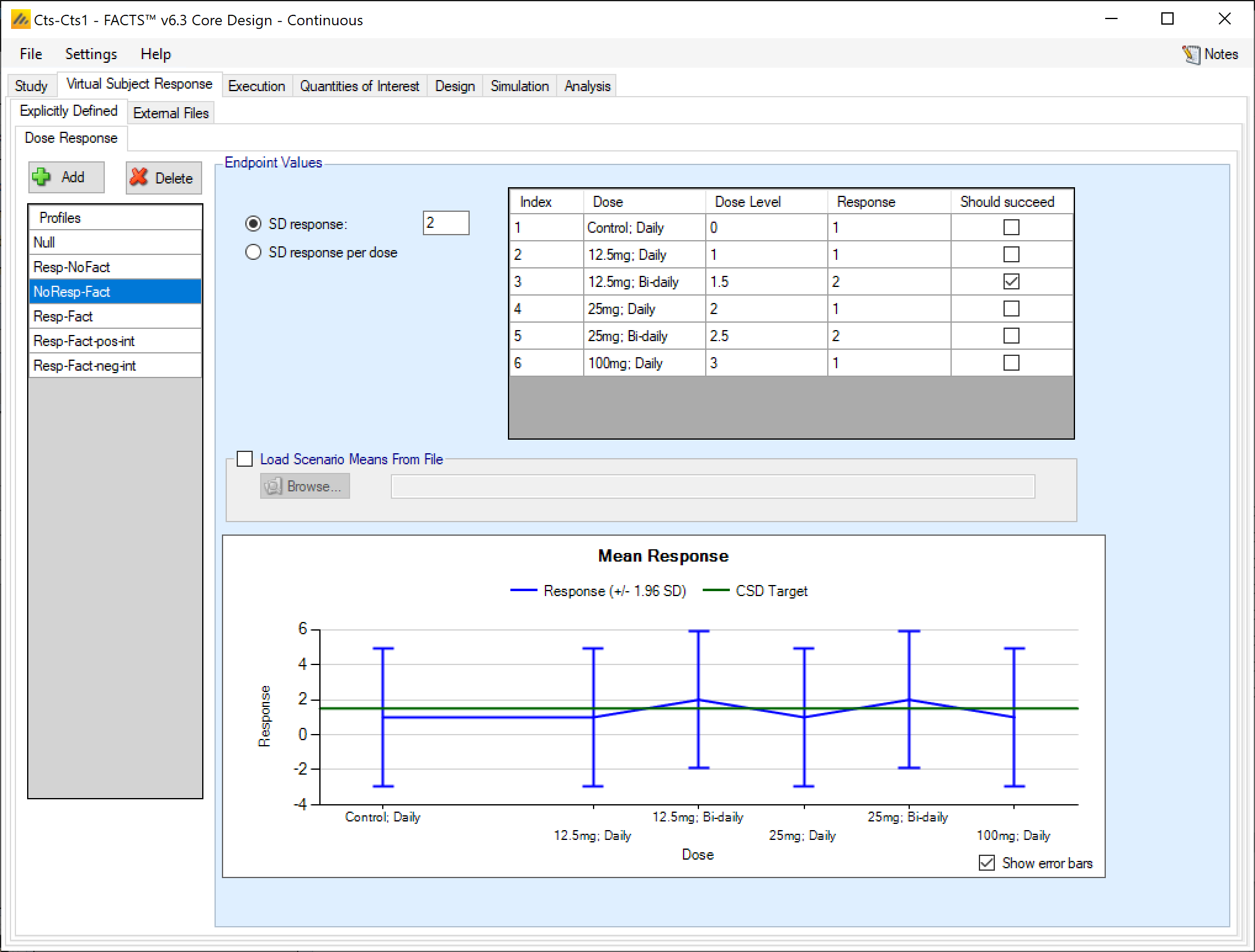
The graph on the Explicitly Defined > Dose Response tab shows the mean response specified for each treatment arm +/- 1.96 SD, and the control response + the default CSD Clinically significant difference level specified on the QOI tab.

If a 2D treatment arm model is being used, the doses are listed in “effective dose strength order” as was defined on the treatment arm tab.

Figure 2: The Explicitly Defined > Dose Response tab when using a 2D treatment arm model.

Load Scenario Means From File

If the “Load scenario means from a file” option is selected, then in scenarios using this profile the simulations will use a range of dose responses instead of what is specified in the table.

Each individual simulation uses one set of mean responses from the supplied file, each row being used in an equal number of simulations. The summary results are thus averaged over all the VSRs in the file. The use of this form of simulation is somewhat different from simulations using a single rate or single external virtual subject response file. When all the simulations are simulated from a single version of the ‘truth’ then the purpose of the simulations is to analyse the performance of the design under that specific circumstance. When the simulations are based on a range of ‘truths’ then the summary results show the expected probability of the different outcomes for the trial over that range of possible circumstance. Note that, to give different VSRs different weights of expectation, the more likely VSRs should be repeated within the file.

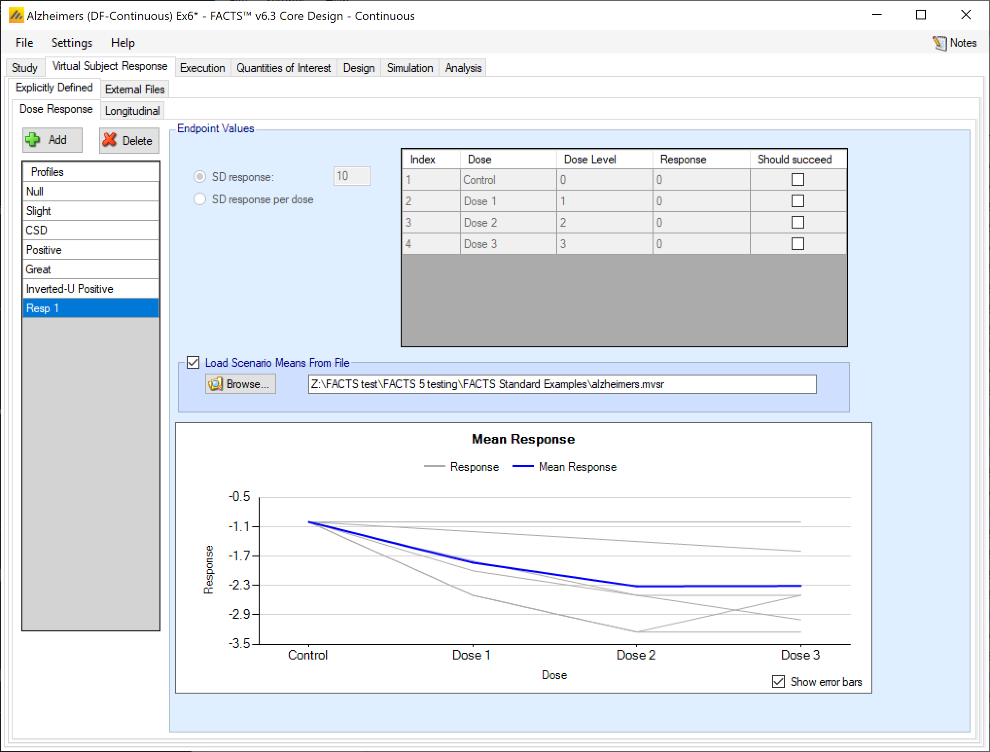
Figure 3: The Explicitly Defined > Dose Response tab when loading scenario means from a file.

After selecting the “.mvsr” file the graph shows the individual mean responses and the overall mean response over all the VSRs.

The format of the file is a simple CSV text file. Lines starting with a ‘#’ character are ignored so the file can include comment and header lines. There must be two columns per treatment arm giving the mean and SD of the change from baseline on each arm, the columns must be grouped first means then SDs and within each group they must be in dose index order. E.g.:

#Cntrl, D1, D2, D3, Cntrl, D1, D2, D3
-1, -1, -1, -1, 5, 5, 5, 5
-1, -1.2, -1.4, -1.6, 5, 5, 5, 5
-1, -1.8, -2.5, -2.5, 5, 5, 5, 5
-1, -2, -2.5, -3, 5, 5, 5, 5
-1, -2.5, -3.25, -3.25, 5, 5, 5, 5
-1, -2.5, -3.25, -2.5, 5, 5, 5, 5

Longitudinal VSR

The explicitly defined virtual subject longitudinal responses can be specified with any of 3 methods. No matter which longitudinal VSR simulation method is selected, it can be combined with any Dose Response VSR, and the dose response VSR is guaranteed to have the marginal distribution Unless Use Baseline Adjustment for Subject Response is specified in the Baseline VSR tab. specified in the dose response VSR section. The longitudinal VSR determines how to correlate early endpoint values with the final endpoint value.

The three longitudinal VSRs available for continuous endpoints are:

Correlated
Hierarchical, which comes in two ‘flavors’:
1. Hierarchical (as in versions of FACTS prior to 6.1): the per subject random element ‘delta’ is scaled at visit ‘t’ by the response fraction f_t at that visit.
2. Hierarchical MMRM (first available in FACTS 6.1): the per subject random element ‘delta’ is the same at all visits.
ITP

Correlated Simulation of Longitudinal Data

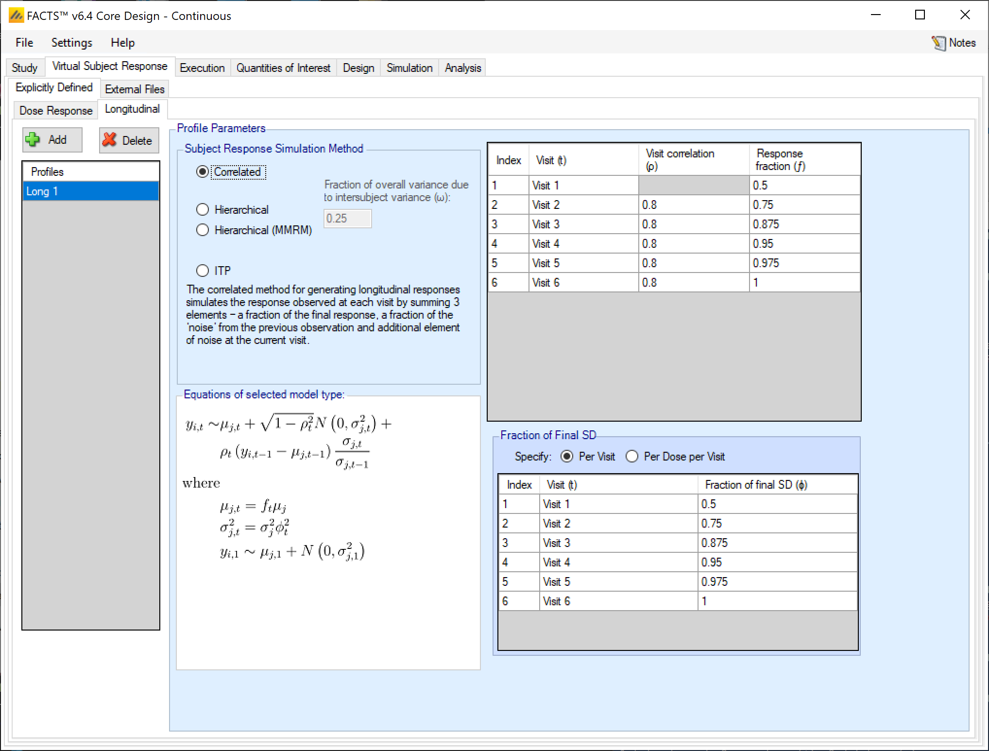
The Correlated method for generating longitudinal responses simulates the response observed at each visit by summing 3 elements – a fraction of the final response, a fraction of the ‘noise’ from the previous observation, and additional element of noise at the current visit.

Figure 4: The Longitudinal VSR tab when specifying the Correlated continuous longitudinal VSR.

The user specifies:

\(\rho_{t}\): the correlation in the observation at visit \(t\) with visit \(t - 1\). Values should be in the range 0-1. The closer to 1, the greater the correlation between visit \(t - 1\) and visit \(t\). The \(\rho\) at Visit 1 is not enterable, because there is no previous visit to correlate the first visit value with.
\(f_{t}\): the fraction of the final mean response \(\mu_{j}\) seen at visit \(t\). Values can lie outside the range 0-1.
\(\varphi_{t}^{2}\): the fraction of the final standard deviation (SD) that will be observed at this visit. Values must be \(>0\). An additional element of noise at visit \(t\) is sampled so that in combination with the noise carried forward from visit \(t - 1\), the overall variance in observations at visit \(t\) will have this fraction of the final variance.

For the first visit of patient \(i\), the response \(y_{i,1}\) assuming patient \(i\) was randomized to dose \(j\) is simulated as:

\[y_{i,1}\ \sim\ N\left( \mu_{j,1},\sigma_{j,1}^{2} \right)\]

For time points after the first visit, observed data is simulated as:

\[y_{i,t}\ \sim\ \mu_{j,t} + \sqrt{1 - \rho_{t}^{2}}N\left( 0,\sigma_{j,t}^{2} \right) + \rho_{t}\left( y_{i,t - 1} - \mu_{j,t - 1} \right)\frac{\sigma_{j,t}}{\sigma_{j,t - 1}} \text{ for } t \geq 2.\]

There are 3 components of this equation. First, is the marginal mean of the response at the particular visit \(t\). This parameter is called \(\mu_{j,t}\). \(\mu_{j,t}\) is simply the dose response at the final endpoint times the proportion of the final effect that should be observed at visit \(t\).

\[\mu_{j,t} = f_{t}\mu_{j}\]

where \(f_{t}\) is input as the response fraction for each visit, and \(\mu_{j}\) is the dose response for dose \(j\), which is input as the Response for each dose on the Dose Response tab.

The second component controls the adjustment of the variance based on the correlation of the endpoint to be sampled with the previous visit’s response. A strong correlation (\(\rho_{t}\) close to \(\pm 1\)) results in a variance reduction term \(\sqrt{1 - \rho_{t}^{2}}\) close to 0, which guarantees that the time \(t\) response is very close to the time \(t - 1\) response. The variance reduction term modifies a dose’s marginal visit variance \(\sigma_{j,t}^{2}\). This dose by visit variance is calculated by squaring the marginal standard deviation for a dose’s final endpoint response \(\sigma_{j}\) times the proportion of the total variance that is observed at visit \(t\), \(\phi_{t}\), which is a user input on the Longitudinal VSR tab.

So, \(\sigma_{j,t}^{2} = \phi_{t}^{2}\sigma_{j}^{2}\) where \(\phi_{t}\) is the fraction of final SD specified in the Longitudinal VSR tab in FACTS, and \(\sigma_{j}\) is the SD of the response specified in the Dose Response VSR tab in FACTS.

The final component of the model adjusts the mean of the visit \(t\) response that is to be simulated based on the residual of the time \(t - 1\) response. This component is:

\[\rho_{t}\left( y_{i,t - 1} - \mu_{j,t - 1} \right)\frac{\sigma_{j,t}}{\sigma_{j,t - 1}}\]

Values of \(\rho_{t}\) close to 1 lead to visit \(t\) responses with Z-scores similar to the visit \(t - 1\) responses, values of \(\rho_{t}\) close to 0 lead to simulation of visit \(t\) responses with no regard to the previous visit’s residual value, and values of \(\rho_{t}\) close to -1 lead to visit \(t\) responses with Z-scores that are -1 times the previous visit’s Z-score.

The specification of the visit level means \(\mu_{j,t}\ \)and variances \(\sigma_{j,t}^{2}\) as response fractions and fractions of final SD, respectively, allows for each created longitudinal VSR to work with every created Dose Response VSR.

Hierarchical model

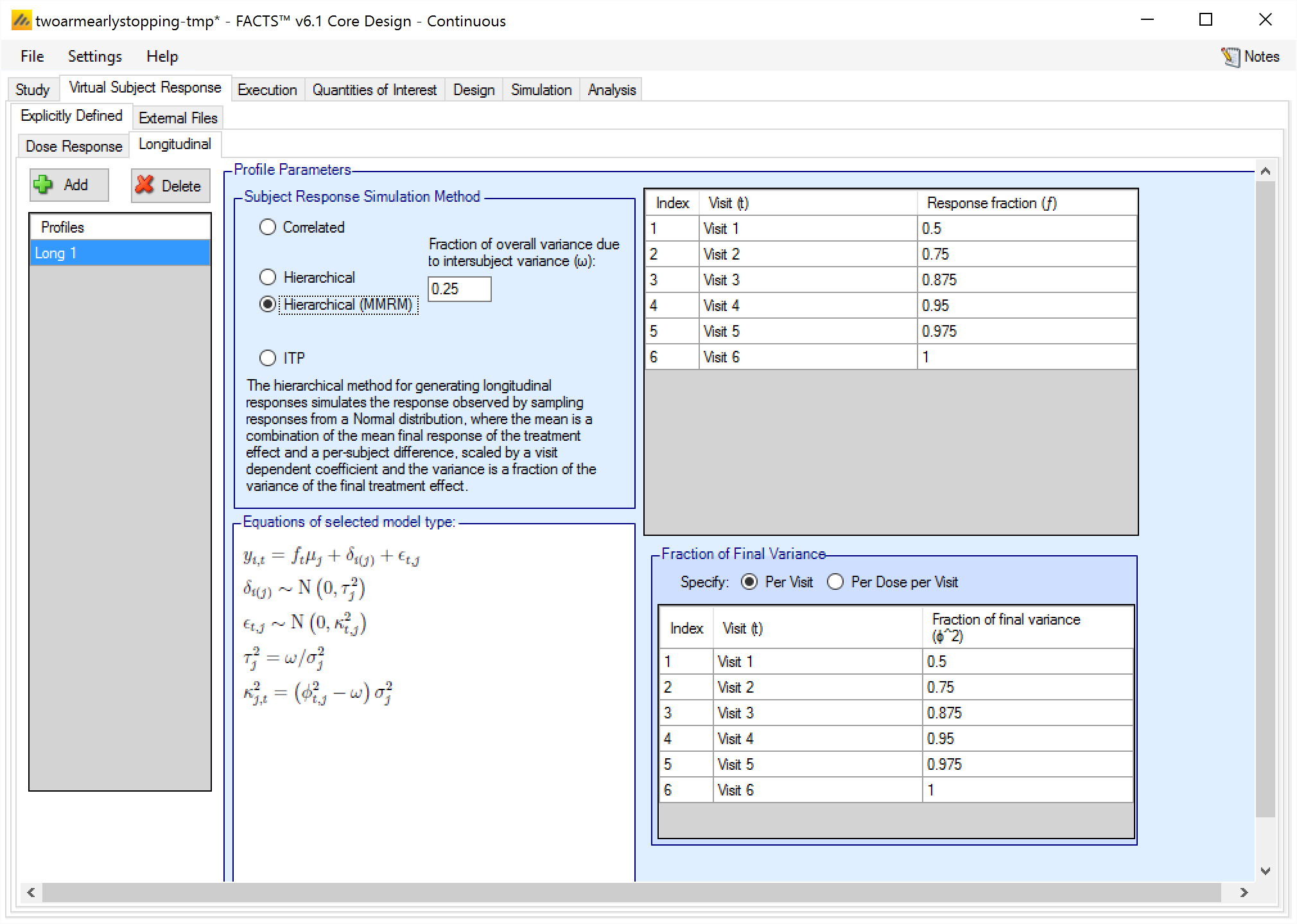
The hierarchical method for generating longitudinal responses simulates the response observed by sampling responses from a Normal distribution, where the mean is a combination of the mean final response of the treatment and a per-subject difference, scaled by a visit dependent coefficient, and the variance is a fraction of the variance of the final treatment effect.

This Hierarchical form of this model has a per-subject random effect parameter \(\delta_{i}\) that is scaled down by the response scaling parameter \(f_{t}\). In the very similar Hierarchical (MMRM) model (described below), the random effect \(\delta_{i}\) is not scaled by \(f_{t}\), so it provides a constant adjustment to all visits.

Figure 5: The Longitudinal VSR tab when specifying the Hierarchical (MMRM) continuous longitudinal VSR.

In the Hierarchical longitudinal subject data simulation model, the response variance is decomposed into two components. One is the within-subject variability (called intra-subject variability), and the other is across-subject variability (Called inter-subject variability). The parameter \(\omega\) determines how much of the total variability is simulated in the inter- and intra-subject variabilities. More variability in the inter-subject simulation means that there is less variability in the intra-subject simulation, so the early visit endpoints will be more correlated with the final visit endpoint, and vice versa.

The parameters of the Hierarchical longitudinal subject data simulation model are:

\(\omega\): the fraction of the variance of the final response (\(\sigma_{j}^{2}\)) on the treatment arm that will be simulated in the inter-subject variance. The higher this value is, the more predictive a subject’s early observations are of their final outcome.
\(f_{t}\): the fraction of the final mean response \(\mu_{j}\) seen at visit \(t\). Values can lie outside the range 0-1.
\(\phi_{jt}^{2}\): the fraction of the final endpoint variance that will be observed at this visit. Values must be \(>0\) and must be such that \(\phi_{jt}^{2} - f_{t}^{2}\omega\) is \(>0\).

Observation \(y_{it}\) is the visit response at visit \(t\) for a subject \(i\) that was randomized from dose \(j\). The observation is generated from the distribution described by:

\[y_{i,t} = f_{t}\left( \mu_{j} + \delta_{i} \right) + N\left( {0,\ \left( \phi_{jt}^{2} - f_{t}^{2}\omega \right)\ \sigma}_{j}^{2} \right)\]

where \(\sigma_{j}^{2}\) is the variance of the final endpoint response for dose \(j\), \(\phi_{jt}^{2}\) is the fraction of total variance observed at visit \(t\) on dose \(j\), \(\mu_{j}\) is the final endpoint response mean for dose \(j\), \(\delta_{i}\) is a subject level random effect, \(f_{t}\) is the fraction of the final endpoint response that is observed at visit \(t\), and \(\omega\) is the proportion of overall variance due to intersubject (across subject) variability.

The prior for the patient random effect term of patient \(i\) who was randomized to dose \(j\) is

\[\delta_{ij}\ \sim\ N\left( 0,\ \omega\sigma_{j}^{2} \right)\]

If \(\omega\) is close to 1, then most of the variability in the responses comes from differences in participants and the visit-to-visit correlation within a participant’s follow-up is high. If \(\omega\) is close to 0, then there is little correlation between visits within a participant’s follow-up, and most of the overall variance comes from noise in the within patient responses, rather than differences across patients. In other words, large values of \(\omega\) lead to early data that is more predictive of the final endpoint.

Note that, in this model the response fraction \(f_{t}\) is multiplied by both the final endpoint mean and the patient level random effect. This results in the variance of the dose \(j\) response at visit \(t\) being \[{\left( \phi_{jt}^{2} - f_{t}^{2}\omega \right)\sigma}_{j}^{2} + f_{t}^{2}\omega\sigma_{j}^{2} = \phi_{jt}^{2}\sigma_{j}^{2}.\]

Additionally, since \(f_{t}\) changes the proportion of the overall variance that comes from the random effect, the simulated correlation between visits decreases when values of \(f_{t}\) less than 1 are provided. See the MMRM version of the Hierarchical simulation model if this is undesirable.

If all \(\phi_{jt}^{2} = 1\) and \(f_{t} = 1\), then the visits will have pairwise correlations equal to \(\omega\). If the \(\phi_{jt}^{2}\) or \(f_{t}\) are less than 1, then the visit pairwise correlations will depend on the input variance fractions \(\phi_{jt}^{2}\) and \(f_{t}\).

Hierarchical (MMRM) model

The Hierarchical (MMRM) longitudinal patient simulation model is very similar to the Hierarchical simulation method, except that in the MMRM version the response fraction for a visit does not modify the patient level random effect. The user inputs for the Hierarchical (MMRM) model are nearly identical to the plain Hierarchical model.

\(\omega\): the fraction of the variance of the final response on the treatment arm (\(\sigma_{j}^{2}\)) that will be simulated in the inter-subject variance. The higher this value is, the more predictive a subject’s early observations are of their final outcome.
\(f_{t}\): the fraction of the final mean response \(\mu_{j}\) seen at visit \(t\). Values can lie outside the range 0-1.
\(\phi_{jt}^{2}\): the fraction of the final endpoint variance that will be observed at this visit for dose \(j\), values must be >0 and must be such that \(\phi_{jt}^{2} - \omega\) > 0.

The Hierarchical MMRM method simulates responses at visit \(t\) for a subject \(i\) that was randomized to dose \(j\) from the distribution:

\[y_{i,t} = f_{t}\mu_{j} + \delta_{i} + N\left(0,\ \left( \phi_{jt}^{2} - \omega \right)\ \sigma_{j}^{2} \right)\].

The prior for the patient random effect term of patient \(i\) who was randomized to dose \(j\) is

\[\delta_{ij}\ \sim\ N\left( 0,\ \omega\sigma_{j}^{2} \right)\]

If \(\omega\) is close to 1, then most of the variability in the responses comes from differences in participants and the visit-to-visit correlation within a participant’s follow-up is high. If \(\omega\) is close to 0, then there is little correlation between visits within a participant’s follow-up, and most of the overall variance comes from noise in the within patient responses rather than differences across patients. In other words, large values of \(\omega\) lead to early data that is more predictive of the final endpoint.

Note that, in this model the response fraction \(f_{t}\) is multiplied by only the final endpoint mean and not the patient level random effect. This results in the variance of the dose \(j\) response at visit \(t\) being \[{\left( \phi_{jt}^{2} - \omega \right)\sigma}_{j}^{2} + \omega\sigma_{j}^{2} = \phi_{jt}^{2}\sigma_{j}^{2}.\]

This total variance is the same as the non MMRM Hierarchical method, but only the \(\phi_{jt}^{2}\) parameter effects the variance of early endpoint responses. If all \(\phi_{jt}^{2} = 1\), then the visits will have pairwise correlations equal to \(\omega\). If the \(\phi_{jt}^{2}\) are less than 1, then the visit pairwise correlations will be larger than \(\omega\), with the exact value depending on the input variance fractions \(\phi_{jt}^{2}\).

Integrated Two Component Prediction (ITP) Simulation of Longitudinal Data

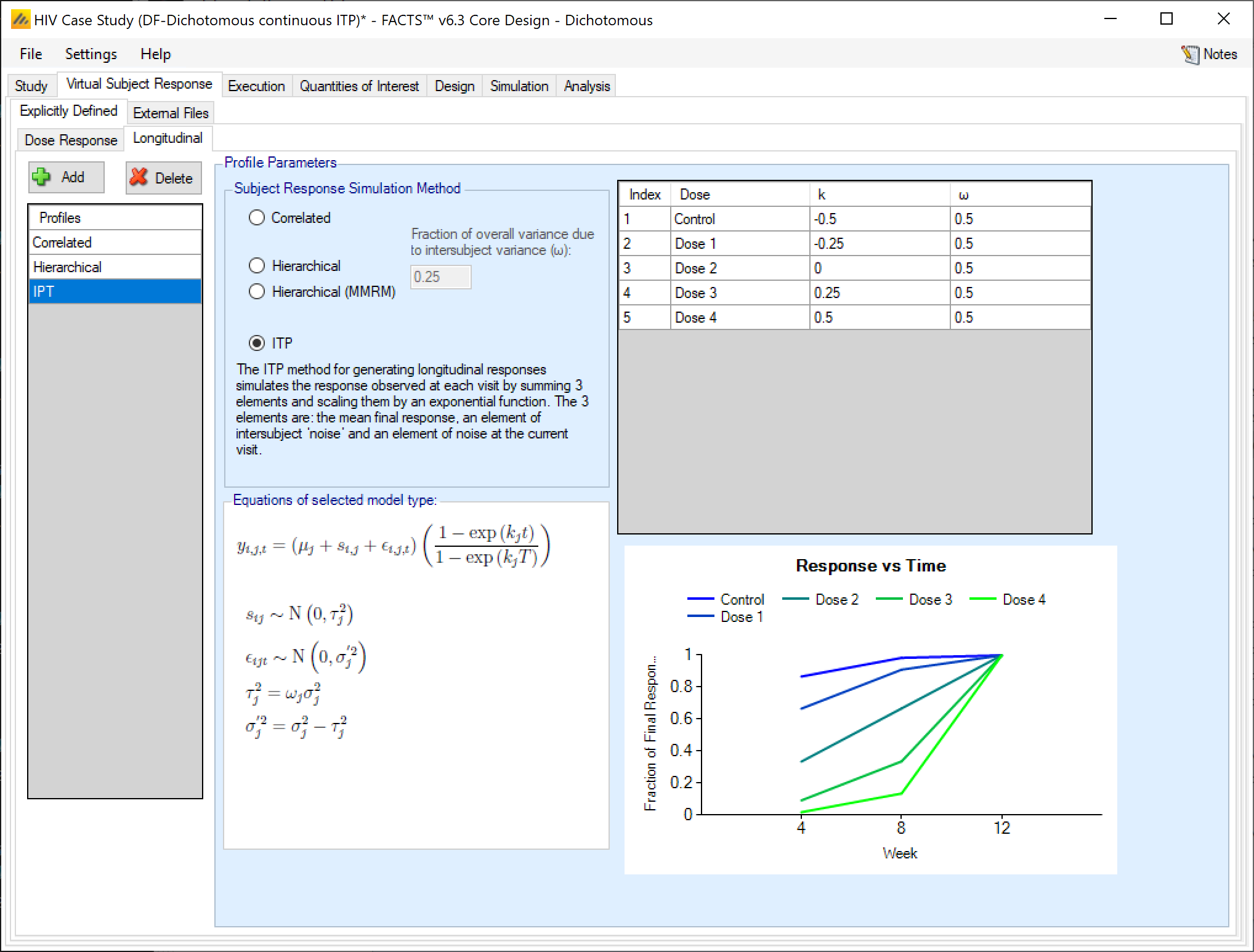
The ITP method for generating longitudinal responses simulates the response observed at each visit by summing 3 elements and scaling them by an exponential function. The 3 elements are: the mean final response, an element of inter-subject variability, and a residual variability at the current visit.

Figure 6: The Longitudinal VSR tab when specifying the ITP continuous longitudinal VSR.

The user specifies

\(\omega_{j}\): fraction (for each dose) of the variance of the final response on the treatment arm (\(\sigma_{j}^{2}\)) used for the inter-subject variance. The higher this value is, the more predictive a subject’s early observations are of their final outcome.
\(k_{j}\): the shape parameter (for each dose) of the exponential component governing the increase in the observed response. The values of \(k\) should be scaled to take into account the length of time (in weeks) to the intermediate and final visits. See below for more intuition on sensible values of \(k\).

For subject \(i\) at visit \(t\), who was randomized to dose \(j\), the response \(y_{it}\) is simulated as:

\[y_{it} = \left( \mu_{j} + s_{i} + \epsilon_{it} \right)\left( \frac{1 - \text{exp}\left( k_{j}x_{t} \right)}{1 - \text{exp}\left( k_{j}x_{T} \right)} \right)\]

where \(\mu_{j}\) is the mean of the final endpoint on dose \(j\), \(s_{i}\sim N\left( 0,\ \omega_{j}\sigma_{j}^{2} \right)\) is a subject specific random effect, each \(\epsilon_{it}\sim N\left( 0,{\ \sigma}_{j}^{2}\left( 1 - \omega_{j} \right) \right)\) is a residual error, \(k_{d}\) is a shape parameter, \(x_{t}\) are the visit times that the \(y_{it}\) are observed, and \(x_{T}\) is the time of the final endpoint.

The ITP model implies that the variance of the observations shrinks towards 0 with the mean (so early visits have reduced expected responses and variances).

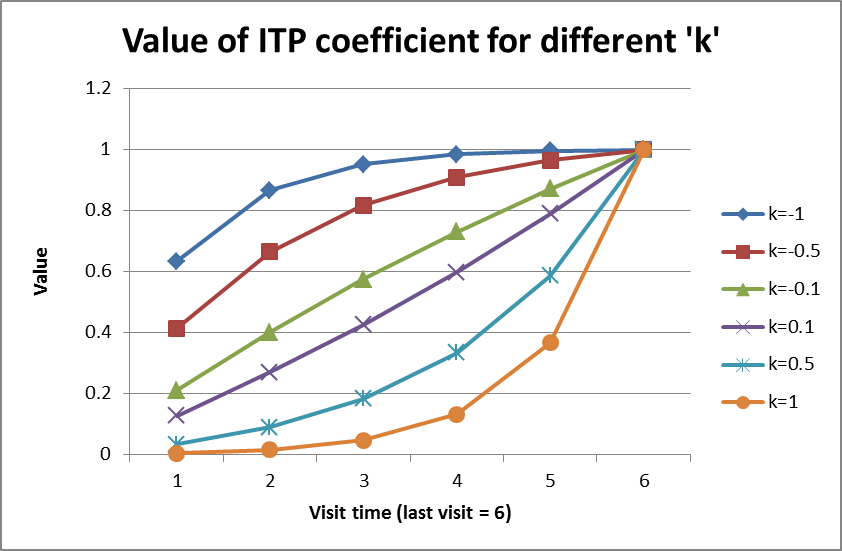
The shape parameter \(k\) determines the rate at which the final endpoint’s eventual effect is observed during a subject’s follow-up. A value of \(k = 0\) indicates that the proportion of effect observed moves linearly with time. A value of \(k < 0\) means that the eventual final effect is observed earlier in follow-up and plateaus off as time moves towards the final endpoint. A value of \(k > 0\) indicates that less of the total final endpoint effect is observed early in follow up, but as time approaches the final endpoint time the proportion of the effect observed increases rapidly. Values of \(k\) less than 0 tend to be more common than values of \(k\) greater than 0. See the figure below for a collection of possible shapes of the change in response using different values of \(k\).

Additionally, unlike the Correlated or Hierarchical simulation methods, the ITP method uses the actual visit time to simulate subject values.

Figure 7: The relationship across intermediate visit means for different shape parameters \(k\).

Baseline VSR

If simulation of baseline has been included on the Study > Study Info tab, a new virtual subject response tab is available for specifying the baseline score.

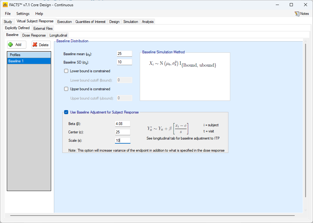
The simulation of distribution of baseline scores is specified using a normal distribution with user specified mean and standard deviation, and optionally applied upper and lower bounds to reflect limitations on the score range or screening criteria. If the simulated baseline score is truncated, then the true mean and SD of the baseline are likely to be different from these values of the mean and SD which are before truncation.

If the response is chosen to be change from baseline on the Study Info tab, then the dose response VSR is specified as change from baseline, and the raw endpoint for a subject will actually be their baseline value plus their simulated change from baseline value. If the response is chosen to be Final endpoint value on the Study Info tab, then the dose response VSR specifies the direct distribution that the final endpoint will be sampled from, and changing the baseline distribution does not effect the final endpoint distribution.

Whether the final endpoint is change from baseline or final endpoint value, it is possible to adjust the final response based on the simulated baseline value. To do so, the user selects “Use Baseline Adjustment for Subject Response” and supplies 3 parameters:

\(\beta\): a coefficient that reflects the degree of influence of baseline on final score and the degree of variability in the final score due to baseline.
c: a centering offset, typically the expected mean of the observed baseline scores
s: a scaling element, typically set to the expected SD of the baseline.

Be aware that performing a baseline adjustment for subject response can change the marginal distribution of the dose response VSR.

Example

In the above screenshot a baseline of mean 25 and SD 10 has been specified for the distribution of the baseline values, so a centering of \(c=25\) and scaling of \(s=10\) is used. Wishing to simulate an overall SD of 5 in the final change from baseline and apportion two-thirds the variance to baseline, \(\beta\) has been set as follows:

The desired final variance is 25 (\(5^2\)), divided into 1/3 dose response and 2/3 baseline effects.
The SD of the simulated response is set to \(\sqrt{\left( 25*\frac{1}{3} \right)} = 2.89\)
The SD of the scaled baseline score is 1, so to contribute half the final variance of 25, Beta is set to \(\sqrt{\left( 25*\frac{2}{3} \right)} = 4.08\)
Note that when simulating a baseline effect in this way, limiting the range of baseline by specifying upper and lower cut-offs – which might be natural limits of the endpoint, or due to inclusion / exclusion criteria in the protocol – can significantly reduce the variance in the final endpoint due to the baseline effect.

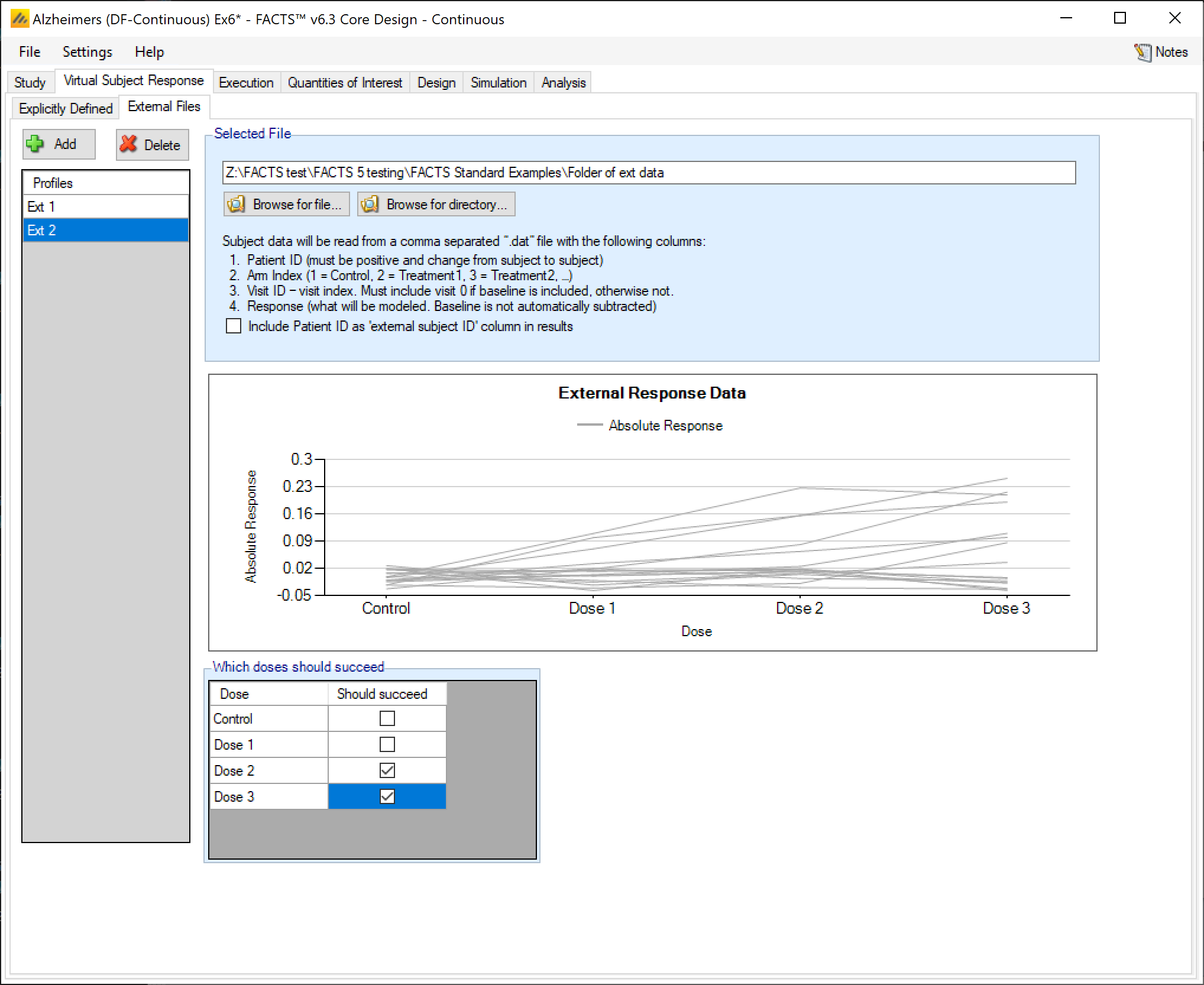
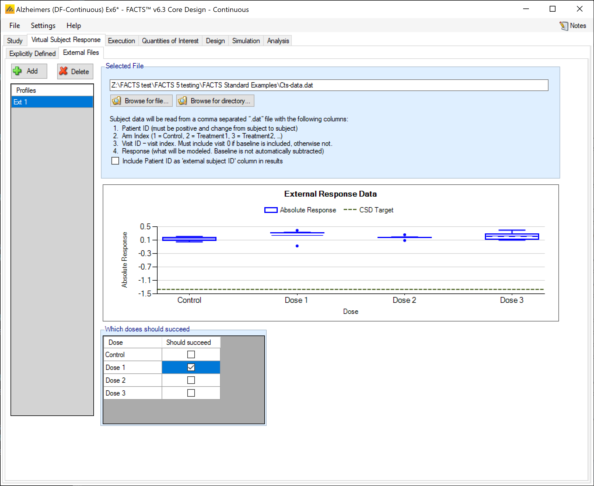
External Files VSR

As well as simulating subject responses within FACTS they can be simulated externally, and imported into FACTS where the supplied responses are sampled from when simulating the trial. The selection of a file containing subject response data (which must be in the required format) can be done from the External Files sub-tab depicted below.

To import an external file, the user must first add a profile to the table. After adding the profile, the user must click “Browse” to locate the file of externally simulated data. The user will then be prompted to locate the external file on their computer with a dialog box.

As with other virtual subject responses, the user can specify which arms “should succeed” at the bottom of the tab.

Figure 9: The external VSR tab in the Core Continuous engine loading a single VSR from a file.

Required Format of Externally Simulated Detail

The supplied data should be in the following format: an ascii file with data in comma separated value format with the following columns:

Patient id, these must be positive integers and unique
Arm Index (1 = Control, 2 = Treatment1, 3 = Treatment2, …)
Visit ID – visit index (1= first visit, 2= second visit, …). If baseline is included, then baseline is visit 0.
Response
1. If no baseline is included, then the response provided must be change from baseline
2. If baseline is included, then the response provided must be the absolute response (and the design engine will compute change from baseline or analyze the absolute response as specified by the user on the Study tab).

Subjects need to have unique, positive integer IDs, all records for each subject should be contiguous and in visit order.

The GUI requires that the file name has a “.dat” suffix.

Below are two examples of files providing externally simulated patient data for 3 subjects with 4 post baseline visits. The No Baseline tab of the table shows an example file for a trial that does not simulate the baseline value, and the With Baseline tab shows an example file for a trial that does simulate the baseline visit.

Note that the first line in both tabs contains column names, and that the row begins with a pound sign (#). This pound sign tells FACTS that it should not try to read that row in as data.

No Baseline
With Baseline

#subj id, Arm ID, Visit ID, Response

1, 1, 1, 0.11
1, 1, 2, 0.22
1, 1, 3, 0.21
1, 1, 4, 0.19
2, 1, 1, 0.09
2, 1, 2, 0.12
2, 1, 3, 0.19
2, 1, 4, 0.22
3, 1, 1, 0.01
3, 1, 2, 0.02
3, 1, 3, 0.05
3, 1, 4, 0.09

#subj id, Arm ID, Visit ID, Response

1, 1, 0, 0.06022
1, 1, 1, 0.12045
1, 1, 2, 0.24091
1, 1, 3, 0.48183
1, 1, 4, 0.60229
2, 1, 0, -0.00586
2, 1, 1, -0.01163
2, 1, 2, -0.02327
2, 1, 3, -0.04654
2, 1, 4, -0.05817
3, 1, 0, 0.01287
3, 1, 1, 0.02574
3, 1, 2, 0.05148
3, 1, 3, 0.10296
3, 1, 4, 0.12870

External Directory of Files

By using the ‘Browse for directory’ option, the user can specify a response profile that comprises a directory containing a number of external response files. Like the “scenario means in a file” option, the files in this directory will be used as a single profile, looping through the different files for successive simulations. So individual simulations will use a single external file from the directory, but the summary results for the scenario will be averaged over all the files, the number of simulations being round down to the nearest multiple of the number of external files in the directory. The format of each individual file should be the same as for a single external file, above. Only files with the “.dat” suffix will be read, other files will be ignored.