The Virtual Subject Response tab allows the user to explicitly define virtual subject response profiles, and/or to import virtual subject response from externally simulated PK/PD data. When simulations are executed, they will be executed for each profile specified by the user.
Explicitly Defined
Unlike other endpoints where simply a response (mean change from base line or rate) is specified, specification of subject responses for a time-to-event endpoint is by separately specifying a piecewise exponential event rate for the control population and then hazard ratios for the treatment arms. For simplicity and consistency, this means of specifying the simulated event rates is also used when no control arm is present and the comparison is with historic control rates.
Control Hazard Rates
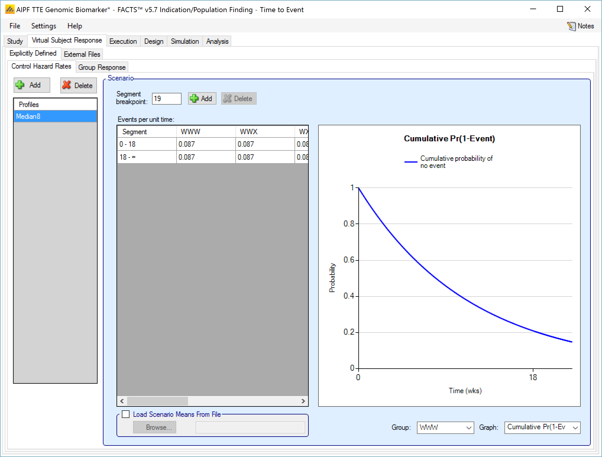
Control hazard rate profiles may be added, deleted, and renamed using the table and corresponding buttons on the left hand side of the screen in Figure 1. Event rates values are entered for control subjects in each group. By specifying segment breakpoints (in weeks) different event rates for different periods of follow-up can be specified. The graphical representation of these values updates accordingly.
To remove an unwanted segment breakpoint, select the row where the segment starts with that breakpoint and click on ‘Delete’. Note that segments are always defined in weeks. The selection of the unit time only applies to the specification of the event rate on this page.
Group Response
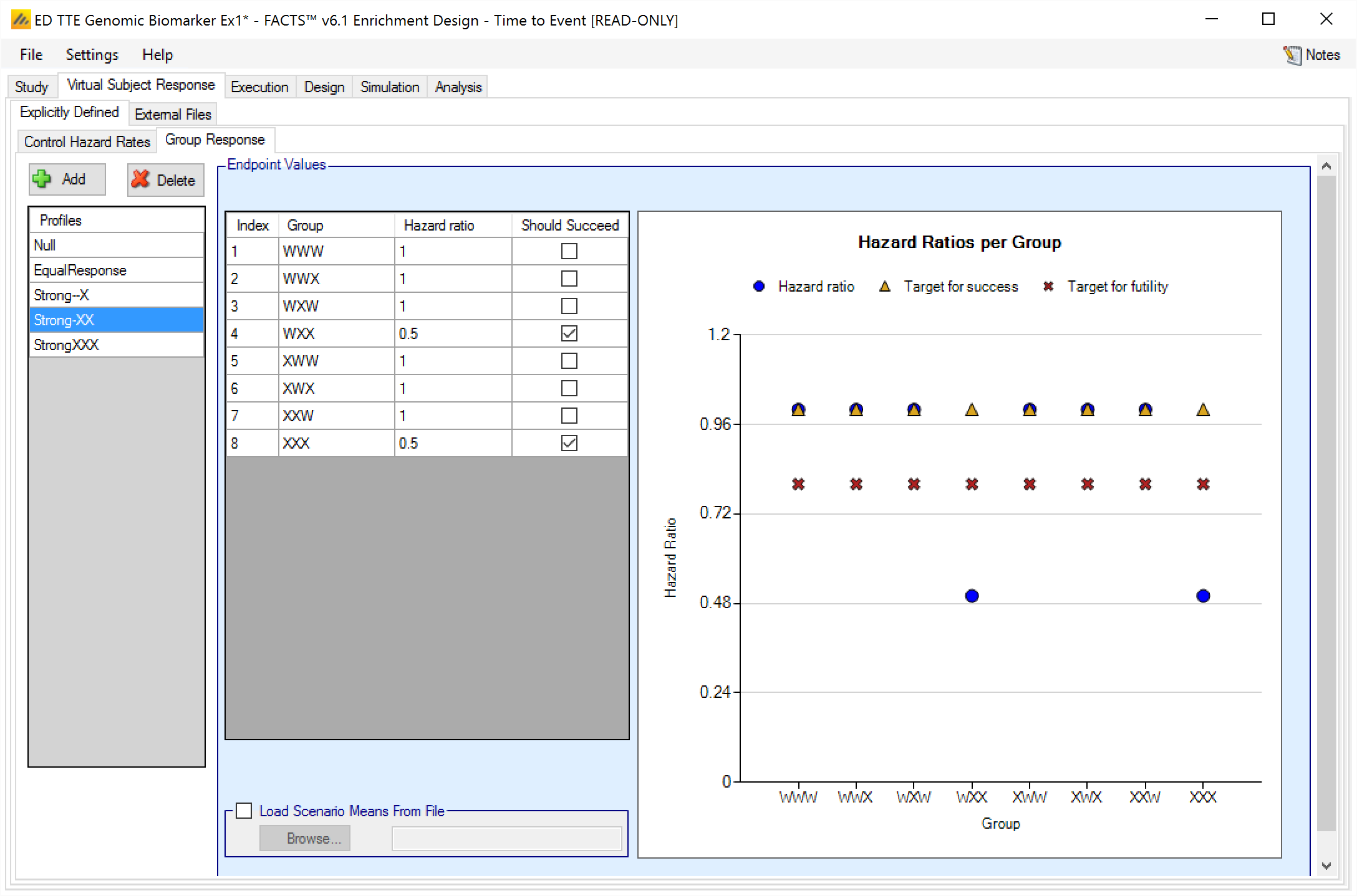
Response profiles may be added, deleted, and renamed using the table and corresponding buttons on the left hand side of the screen in Figure 2. Hazard ratios are entered for the study treatment arm for each group directly into the Hazard ratio column of the table. The graphical representation of these values updates accordingly.
In addition it is possible for the user to specify if a group “Should Succeed” using the “Should succeed” checkbox on each row. This is then used in the summary of the simulation results to compute how often the simulated trial was successful and groups that ‘Should Succeed’ were successful (reported in the column “Ppn Correct Groups”) and how often the simulated trial was successful and groups that were not marked ‘Should Succeed’ were successful (reported in the column “Ppn Incorrect Groups”).
This graph that shows the response to simulate that has been specified – as with all graphs in the application – may be easily copied using the ‘Copy Graph’ option in the context menu accessed by right-clicking on the graph. The user is given the option to copy the graph to their clipboard (for easy pasting into other applications, such as Microsoft Word or PowerPoint), or to save the graph as an image file.
Load Scenario Response From File
If the “Load scenario means from a file” option is selected then in scenarios using this profile the simulations will use a range of dose responses.
Each individual simulation uses one set of responses from the supplied file, each row being used in an equal number of simulations. The summary results are thus averaged over all the VSRs in the file. The use of this form of simulation is somewhat different from simulations using a single rate or single external virtual subject response file. When all the simulations are simulated from a single version of the ‘truth’ then the purpose of the simulations is to analyse the performance of the design under that specific circumstance. When the simulations are based on a range of ‘truths’ loaded from an ‘.mvsr’ file then the summary results show the expected probability of the different outcomes for the trial over that range of possible circumstances. Note that to give different VSRs different weights of expectation, the more likely VSRs should be repeated within the file.
For TTE the user must supply 2 files – one for the Control Hazard Rates and one for the Hazard Ratios in each group. MVSR hazard rates are only combined with MVSR control hazard rates. MVSR hazard rates are only combined with MVSR control hazard rates. The lines from each file are paired up for each simulation, so the first control hazard rate is used with the first group response hazard ratio, the second control hazard rate is used with the second dose response hazard ratio and so on. There must be the same number of lines in each file.
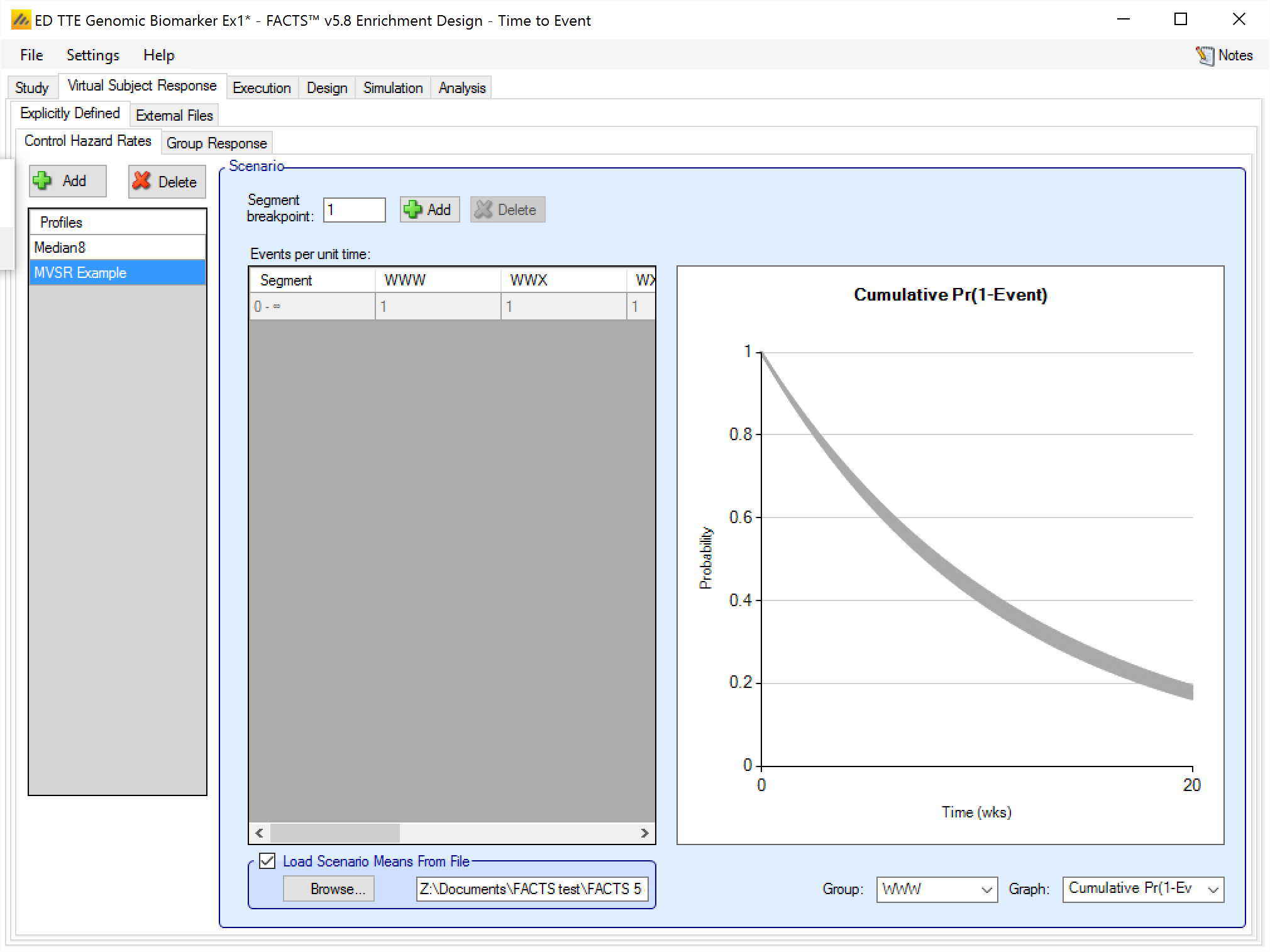
After selecting the “.mvsr” file the graph shows the individual control hazard rates for each group.
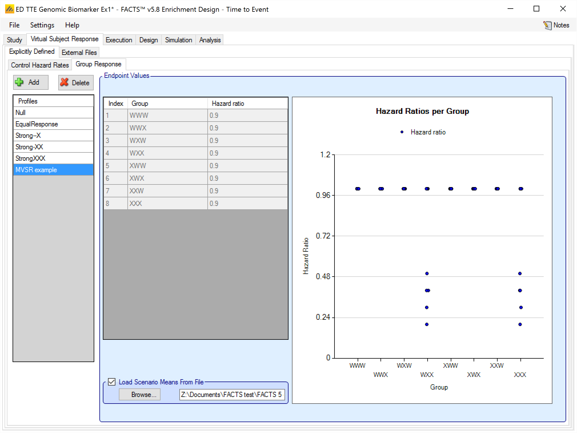
After selecting the “.mvsr” file the graph shows the individual hazard ratios for each group.
The format of the file is a simple CSV text file. Lines starting with a ‘#’ character are ignored so the file can include comment and header lines. The VSR parameters are provided in two separate files, (the number of lines in the files must be the same for the two files). The formats are:
The Control Hazard Rate File: Each line should contain columns [L1,1, L1,2, … , L1,S, L2,1, L2,2, … , L2,S, … LG,1, LG,2, … , LG,S] giving the true control hazard rates (lambda) for each of the S segments for each of the G groups. (Note: FACTS assumes that the unit of time is weeks)
The Hazard Ratio File: Each line should contain columns [HR1, HR2, … , HRG] giving the true treatment arm Mean Hazard Ratios for each of the G groups.
For example:
# TTE control hazard rates, 8 groups 1 segment
# Same number of rows as in Group Response MVSR file
#G1
0.082, 0.087, 0.083, 0.085, 0.091, 0.090, 0.087, 0.087
0.083, 0.086, 0.085, 0.083, 0.090, 0.091, 0.088, 0.087
0.084, 0.085, 0.087, 0.082, 0.089, 0.088, 0.089, 0.087
0.085, 0.084, 0.082, 0.087, 0.088, 0.089, 0.090, 0.087
0.086, 0.083, 0.084, 0.086, 0.087, 0.086, 0.091, 0.087
0.087, 0.082, 0.086, 0.084, 0.086, 0.087, 0.086, 0.087
0.088, 0.091, 0.088, 0.090, 0.085, 0.084, 0.085, 0.087
0.089, 0.090, 0.090, 0.088, 0.084, 0.085, 0.084, 0.087
0.090, 0.089, 0.089, 0.091, 0.083, 0.083, 0.083, 0.087
0.091, 0.088, 0.091, 0.089, 0.082, 0.082, 0.082, 0.087
# TTE 8 Groups, HR for each group
# 5 Null cases
1.0, 1.0, 1.0, 1.0, 1.0, 1.0, 1.0, 1.0
1.0, 1.0, 1.0, 1.0, 1.0, 1.0, 1.0, 1.0
1.0, 1.0, 1.0, 1.0, 1.0, 1.0, 1.0, 1.0
1.0, 1.0, 1.0, 1.0, 1.0, 1.0, 1.0, 1.0
1.0, 1.0, 1.0, 1.0, 1.0, 1.0, 1.0, 1.0
# increasing mixed strong XX
1.0, 1.0, 1.0, 0.2, 1.0, 1.0, 1.0, 0.3
1.0, 1.0, 1.0, 0.3, 1.0, 1.0, 1.0, 0.2
1.0, 1.0, 1.0, 0.4, 1.0, 1.0, 1.0, 0.4
1.0, 1.0, 1.0, 0.4, 1.0, 1.0, 1.0, 0.5
1.0, 1.0, 1.0, 0.5, 1.0, 1.0, 1.0, 0.4
External
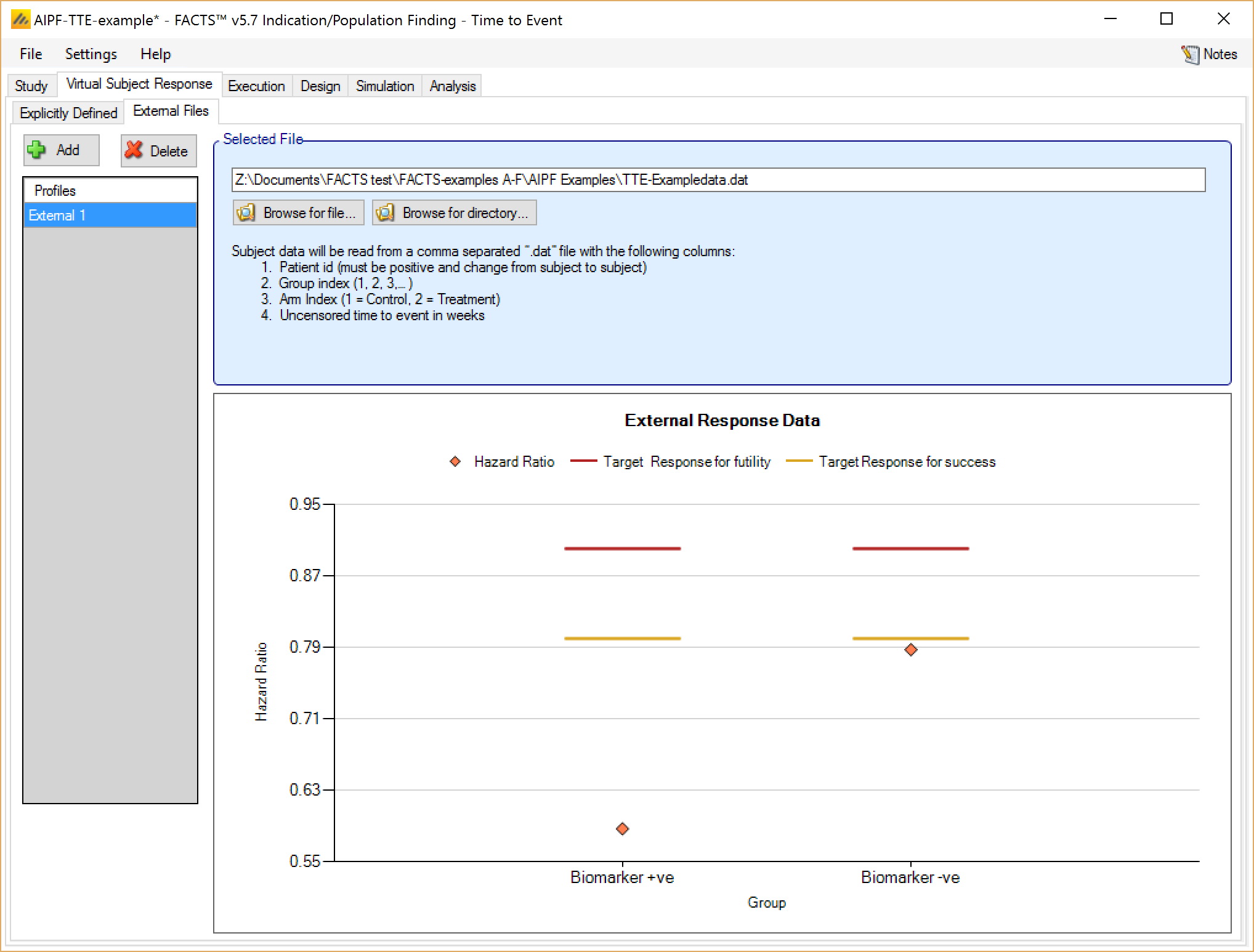
As well as simulating subject response within FACTS they can be simulated externally, from a PK-PD model for instance, and imported into FACTS where the supplied responses are sampled from when simulating the trial. The specification of a file containing subject response data (which must be in the required format) can be done from the External Files sub-tab depicted below.
To import an external file, the user must first add a profile to the table. After adding the profile a file selector window is opened and the user must select the file of externally simulated data. To change the selection, click the ‘Browse’ button .
Required Format of Externally Simulated Detail
The supplied data should be in the following format: an ascii file with data in comma separated value format with the following columns:
Patient id
Group index (1, 2, 3,… )
Arm Index (1 = Control, 2 = Treatment)
Uncensored time to event in weeks
The GUI requires that the file name has a “.dat” suffix.
The following shows values from an example file. Unlike other endpoints there is only one line per subject, as there is no need to record the subject’s state at interim visits.
#Patient ID, Group Index, Arm Index, Time to Event
1, 1, 1, 8.87
2, 1, 2, 9.34
3, 2, 1, 6.78
4, 2, 1, 10.23
5, 2, 1, 9.96
6, 2, 2, 5.6
7, 1, 1, 37.01
8, 1, 2, 28.67
9, 1, 1, 39.70
Simulated subjects will be drawn from this supplied list, with replacement, to provide the simulated response values.