In FACTS Core with a dichotomous endpoint there are 4 different ways to specify the virtual subject response:
Explicit specification of a dichotomous endpoint
Explicit specification of a restricted Markov endpoint
Explicit specification of a continuous endpoint that is dichotomized into responder / non-responder based on the response at the final visit.
Importation of an externally generated set of simulated subject results.
Explicitly Defined Dichotomous Response
Explicitly defined VSRs are the most common type specified in FACTS. In dichotomous endpoint designs, an explicitly defined VSR is specified by providing a response rate for each arm in the trial. The dichotomous final outcome will be simulated having the desired response rate, and longitudinal correlation can be simulated connecting subjects’ intermediate endpoints to the final endpoint.
Dose Response
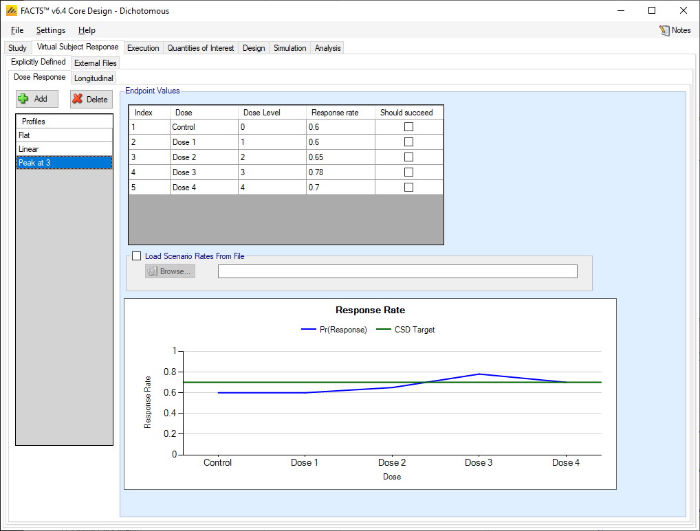
Dose response profiles can be added and deleted, and for each profile the user specifies:
The response rate for each treatment arm.
A check box that allows the user to specify whether a specific arm “should succeed” in that scenario: so that FACTS can report on the proportion of simulations that were successful and a ‘good’ treatment arm selected.
The graph on the tab shows the mean response rate specified and the target.
If a 2D treatment arm model is being used, the doses are listed in “effective dose strength order” as was defined on the treatment arm tab.
Load Scenario Rates From File
If the “Load scenario means from a file” option is selected then in scenarios using this profile the simulations will use a range of dose responses. Each individual simulation uses one set of response rates from the supplied file, each row being used in an equal number of simulations. The summary results are thus averaged over all the VSRs in the file. The use of this form of simulation is somewhat different from simulations using a single rate or single external virtual subject response file. When all the simulations are simulated from one ‘truth’ then the purpose of the simulations is to analyse the performance of the design under that specific circumstance. When the simulations are based on a range of ‘truths’ then the summary results show the expected probability of the different outcomes for the trial over that range of possible circumstances. Note that to give different VSRs different weights of expectation, the more likely VSRs should be repeated within the file.
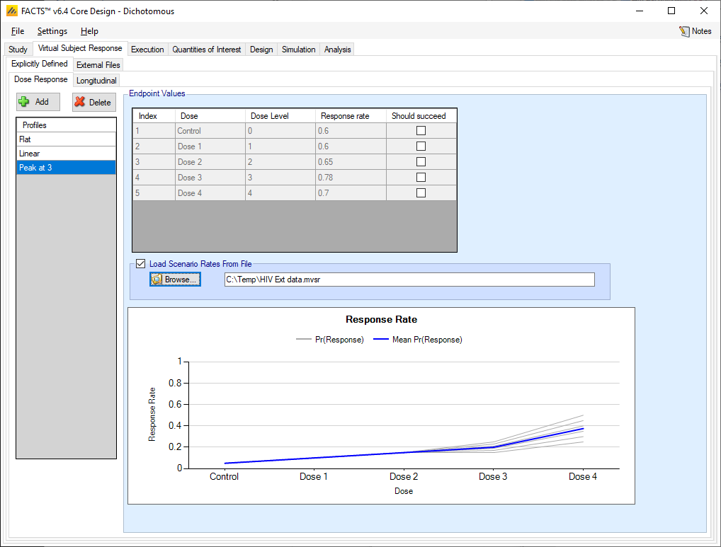
After selecting the “.mvsr” file the graph shows the individual response rates and the mean response rate over all the VSRs.
There is a check box per dose that allows the user to specify whether a specific arm “should succeed” in that scenario: so that FACTS can report on the proportion of simulations that were successful and a ‘good’ treatment arm selected.
The format of the “.mvsr” file is a simple CSV text file. Lines starting with a ‘#’ character are ignored, so the file can include comment and header lines. There must be one column per treatment arm, and they must be in dose index order. Each value is the underlying response rate to simulate. E.g.:
#Cntrl, D1, D2, D3, D4
0.05, 0.1, 0.15, 0.25, 0.5
0.05, 0.1, 0.15, 0.23, 0.45
0.05, 0.1, 0.15, 0.21, 0.4
0.05, 0.1, 0.15, 0.19, 0.35
0.05, 0.1, 0.15, 0.17, 0.3
0.05, 0.1, 0.15, 0.15, 0.25
Longitudinal
The tab for defining dichotomous longitudinal response profiles allows the user to specify the overall transition probabilities between responder and non-responder.
If no special longitudinal options are selected on the Study Info page, then this default simulation method that uses transition probabilities to simulate sequential dichotomous endpoints is used.
The transition probabilities method for generating longitudinal responses simulates the response observed at each visit by using the probability that a subject becomes or remains a ‘1’ from one visit to the next – and all subjects start with a response of 0.
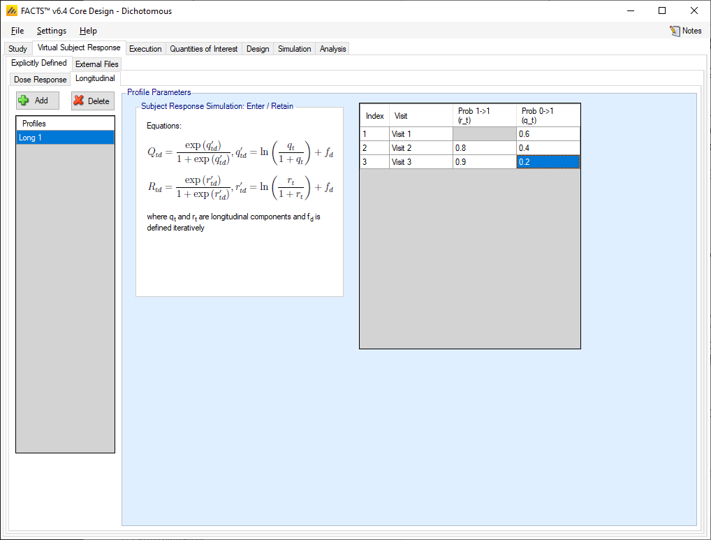
The user specifies for each visit,
the probability of a subject whose response was a ‘0’ at the previous visit having a response of ‘1’ at this visit
the probability of a subject whose response was a ‘1’ at the previous visit having a response of ‘1’ at this visit
However, these probabilities imply a particular probability that a subject has a response of ‘1’ at the final visit, so they need to be modified for each arm in each dose response profile to give the desired final probability of response. This is done by numerically determining for each final response rate, a single value which when added to all the specified transition probabilities in the log-odds space yield the desired probability of final response.
Let \(Q_{td}\) be the probability of transitioning from 0 to 1, and \(R_{td}\) be the probability of transitioning from 1 to 1 for each visit (t) and dose (d).
For the 1st visit:
\[P\left( y_{1d} = 1 \right) = Q_{1d}\]
which is like considering the imaginary 0th visit to have been a non-response. For subsequent visits:
\[P\left( y_{td} = 1 \middle| y_{t - 1,d} = 0 \right) = Q_{td}\]
\[P\left( y_{td} = 1 \middle| y_{t - 1,d} = 1 \right) = R_{td}\]
The dose response (\(P_{d}\)) is first specified in the VSR > Explicitly Defined > Dose Response tab, and then longitudinal components (\(q_{t}\) and \(r_{t}\)) are specified separately. FACTS then makes an adjustment to the longitudinal components \(q_{t}\) and \(r_{t}\) to calculate \(Q_{td}\) and \(R_{td}\) for each dose while maintaining the value for \(P_{d}\) specified in the Dose Response tab.
The matrices Q and R are calculated by applying offsets \(f_{d}\) in log odds space to the longitudinal values:
\[Q_{t,d} = \frac{e^{q'_{td}}}{1 + e^{q'_{td}}}, \ \ q'_{td} = \ln\left( \frac{q_{t}}{1 + q_{t}} \right) + f_{d}\]
\[R_{t,d} = \frac{e^{r'_{td}}}{1 + e^{r'_{td}}}, \ \ r'_{td} = \ln\left( \frac{r_{t}}{1 + r_{t}} \right) + f_{d}\]
where \(f_{d}\) is calculated iteratively for each dose to ensure that Q and R give the correct final probability of response for each dose. As a result,
\[P_{d} = x_{Td}\]
where
\[x_{1d} = Q_{1d}\]
and
\[x_{t} = x_{t - 1}R_{td} + \left( 1 - x_{t - 1} \right)Q_{td}\]
Example
With 3 visits and probabilities of \(0\rightarrow 1\) of \(0.2\) and of \(1\rightarrow 1\) of \(0.9\) at each visit, the probability of a final response is 0.438. This 0.438 is fixed, and cannot be changed without changing the transition probabilities.
| Index | Visit | Prob 1 \(\rightarrow\) 1 (\(r_t\)) |
Prob 0 \(\rightarrow\) 1 (\(q_t\)) |
Cumulative Pr(Resp) |
|---|---|---|---|---|
| 1 | Visit 1 | \(0.2\) | \(0.2\) | |
| 2 | Visit 2 | \(0.9\) | \(0.2\) | \(0.2*0.9\) \(+\;(1-0.2)*0.2\) \(= 0.34\) |
| 3 | Visit 3 | \(0.9\) | \(0.2\) | \(0.34*0.9\) \(+\;(1-0.34)*0.2\) \(= 0.438\) |
If a response profile calls for the probability of a final response to be simulated with a probability of 0.8, a fixed offset in log-odds is found which, when applied to all the transition probabilities, results in the desired final probability of a response. Replicating this by hand to an accuracy of 4 significant digits yields an offset of \(f_d = 1.173\), which gives:
\[\text{logit}^{-1}(\text{logit}(0.2) + 1.173) = 0.4469\] \[\text{logit}^{-1}(\text{logit}(0.9) + 1.173) = 0.9668\]
Then,
| Index | Visit | Prob 1 \(\rightarrow\) 1 (\(r_t\)) |
Prob 0 \(\rightarrow\) 1 (\(q_t\)) |
Cumulative Pr(Resp) |
|---|---|---|---|---|
| 1 | Visit 1 | \(0.4469\) | \(0.4469\) | |
| 2 | Visit 2 | \(0.9668\) | \(0.4469\) | \(0.4469*0.9668\) \(+ (1-0.4469)*0.4469\) \(= 0.6792\) |
| 3 | Visit 3 | \(0.9668\) | \(0.4469\) | \(0.6792*0.9668\) \(+ (1-0.6792)*0.4469\) \(= 0.8000\) |
Explicitly Defined Restricted Markov model
If on the Study > Study Info tab, the special longitudinal option of using the restricted Markov is selected then this tab is available for specifying jointly how subject interim and final outcomes are to be simulated:
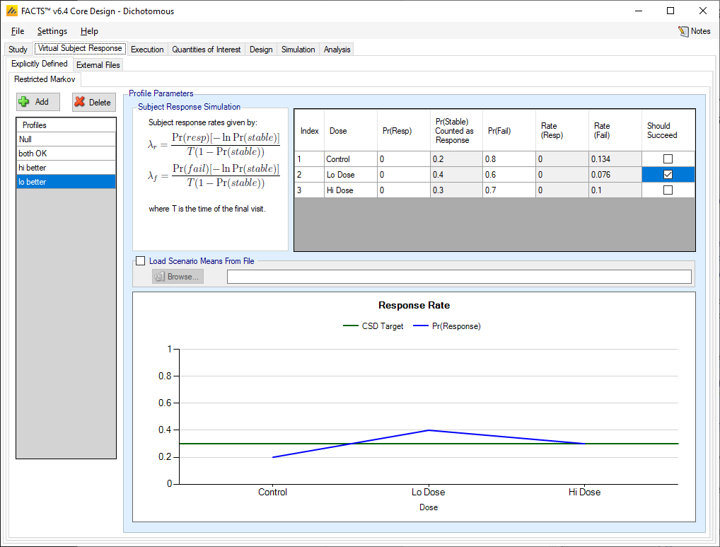
Unlike the simulation of the conventional dichotomous outcome, with Restricted Markov the longitudinal and final response are specified together.
The Absorbing Markov Chain model assumes at each visit patients are in one of three states – responder, stable disease, or failure (non-responder). The responder and failure states are assumed to be absorbing, so patients entering one of these states remain in those states for the duration of the study. Thus, all patient profiles will consist of some duration of stable disease followed by a permanent transition to responder or failure. If a subject remains in the stable state through their final endpoint time, the final response is made dichotomous by the user specifying whether patients in the stable state at the final visit should be classified as responders or failures.
For each dose the user specifies the probability that the subject will be a failure at their final endpoint, and the probability that a subject will be a responder at their final visit. Given these probabilities, FACTS can calculate the probability that a subjects is in the stable state at their final visit, and then the mechanism for generating subjects longitudinal data is:
Two independent exponentially distributed variables, one measuring the time until response \(T_{R}\) and another measuring the time until failure \(T_{F}\), are simulated when the subject enters the study.
If either of variable has a value less than the final endpoint time, the engine determines which variable (\(T_{R}\) or \(T_{F}\)) is the minimum. All visits whose time occurs less than that minimum are stable, while all visits past that variable’s time are classified as that variable’s corresponding state (thus, if visits occur every week for 10 weeks, the response variable \(T_{R}\) is 4.5, and the failure variable \(T_{F}\) is 9.5, then the response variable is the minimum, visits 1-4 are stable, and visits 5-10 are a response.
If neither variable is less than the final endpoint time, the final endpoint and all visits are assumed to be stable.
The parameters of the exponential variables are determined so that they agree with the user entries for the probabilities of response, stable, and failure at the final endpoint. Given T is the time of the final endpoint and a particular dose has probability for response, stable, and failure of Pr(resp), Pr(stable), and Pr(fail) with Pr(stable) strictly between 0 and 1, the appropriate exponential parameters (again there are separate rates in each group and arm) are
\[\lambda_{r} = \frac{\Pr(resp)\left\lbrack - \ln{Pr(stable)} \right\rbrack}{T\left( 1 - Pr(stable) \right)}\] \[\lambda_{f} = \frac{\Pr(fail)\left\lbrack - \ln{Pr(stable)} \right\rbrack}{T\left( 1 - Pr(stable) \right)}\]
If one of these rates is 0, that random variable is removed from the calculation (e.g. if Pr(fail)=0 then failures are not generated). If Pr(stable)=0, the transition to response or failure is assumed to occur instantaneously after enrolment, and thus a weighted coin is flipped with probabilities Pr(resp) and Pr(fail) and all visits are equal to the result (e.g. all visits are responses or all visits are failures depending on the result of that weighted coin flip). If Pr(stable)=1, then all visits are stable.
There is a check box per dose that allows the user to specify whether a specific arm “should succeed” in that scenario so that FACTS can report on the proportion of simulations that were successful and a ‘good’ treatment arm selected.
The graph on the Restricted Markov tab shows the probability of response for each arm and the target CSD relative to the response on control.
Load Scenario Means From File
If restricted Markov is being used, then there must be two sets of columns in the .mvsr column. The first half of the columns gives the overall response rate for each arm, and the second half of columns give the overall failure rate per arm. For example, to specify VSR’s for the restricted Markov model with varying response rates and failure rates constant at 0.1:
#Cntrl, 1mg, 5mg, 10mg, 25mg, 50mg, 100mg, Cntrl, 1mg, 5mg, 10mg, 25mg,
50mg, 100mg
0.2, 0.2, 0.2, 0.2, 0.2, 0.2, 0.2, 0.1, 0.1, 0.1, 0.1, 0.1, 0.1, 0.1
0.2, 0.2, 0.2, 0.17, 0.15, 0.12, 0.1, 0.1, 0.1, 0.1, 0.1, 0.1, 0.1, 0.1
0.2, 0.21, 0.22, 0.23, 0.25, 0.27, 0.28, 0.1, 0.1, 0.1, 0.1, 0.1, 0.1,
0.1
0.2, 0.22, 0.22, 0.27, 0.3, 0.32, 0.35, 0.1, 0.1, 0.1, 0.1, 0.1, 0.1,
0.1
0.2, 0.22, 0.24, 0.28, 0.35, 0.4, 0.4, 0.1, 0.1, 0.1, 0.1, 0.1, 0.1, 0.1
0.2, 0.22, 0.25, 0.35, 0.4, 0.35, 0.3, 0.1, 0.1, 0.1, 0.1, 0.1, 0.1, 0.1
0.2, 0.3, 0.4, 0.35, 0.3, 0.2, 0.15, 0.1, 0.1, 0.1, 0.1, 0.1, 0.1, 0.1
Explicitly Defined Dichotomized Continuous Response
If, on the Study > Study Info tab, the special longitudinal option is selected that the endpoint is a dichotomized continuous response, then instead of using the dichotomous endpoint infrastructure the continuous dose response model and longitudinal data simulation tabs are used. After the final endpoint and all intermediate endpothey are dichotomized using the threshold specified on the Study Info tab. ints are simulated from the continuous distribution,
Load Scenario Means From File
If a dichotomized continuous endpoint is being used then there must be two sets of columns, the first giving the mean change from baseline and the second giving the SD of the change (as in FACTS Core Continuous). For example, with control and 3 doses, and where the SD will be 5 for all doses in all VSRs:
#Means SDs
#Cntrl, D1, D2, D3, Cntrl, D1, D2, D3
-1, -1, -1, -1, 5, 5, 5, 5
-1, -1.2, -1.4, -1.6, 5, 5, 5, 5
-1, -1.8, -2.5, -2.5, 5, 5, 5, 5
-1, -2, -2.5, -3, 5, 5, 5, 5
-1, -2.5, -3.25, -3.25, 5, 5, 5, 5
-1, -2.5, -3.25, -2.5, 5, 5, 5, 5
External
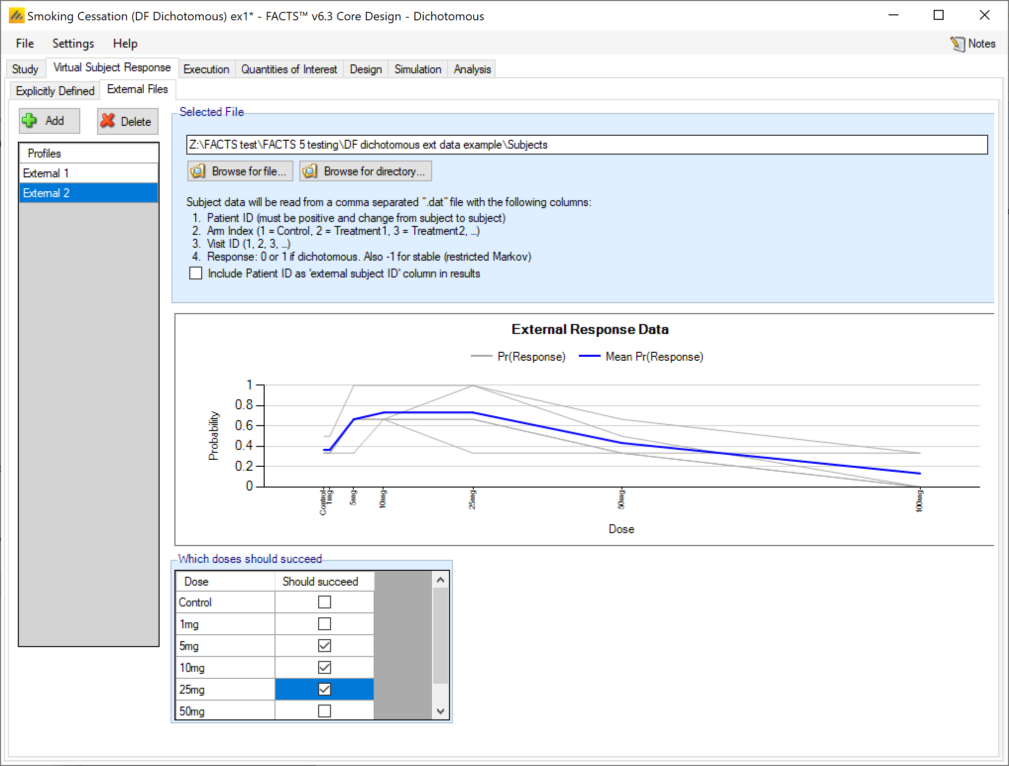
As well as simulating subject responses within FACTS they can be simulated externally, and imported into FACTS where the supplied responses are sampled from with replacement when simulating the trial. The selection of a file containing subject response data (which must be in the required format) can be done from the External Files sub-tab depicted below. The External Files option is available if specifying the dichotomous endpoint as restricted Markov, dichotomized continuous, or without special longitudinal options.
To import an external file, the user must first add a profile to the table. After adding the profile, the user must click “Browse” to locate the file of externally simulated data. The user will then be prompted to locate the external file on their computer with a dialog box.
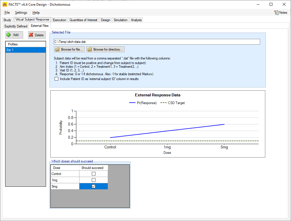
Required Format of Externally Simulated Detail
The supplied data should be in the following format: an ascii file with data in comma separated value format with the following columns:
Patient id – these must be sequential, unique, positive integers.
Arm Index (1 = Control, 2 = Treatment1, 3 = Treatment2, …)
Visit ID – visit index (1 = first visit, 2 = second visit, …)
Response: 0 for no response, 1 for response
Patient id – these must be sequential, unique, positive integers.
Arm Index (1 = Control, 2 = Treatment1, 3 = Treatment2, …)
Visit ID – visit index (1 = first visit, 2 = second visit, …)
Response: 0 for no response, 1 for response, -1 for stable
Patient id - these must be sequential, unique, positive integers.
Arm Index (1 = Control, 2 = Treatment1, 3 = Treatment2, …)
Visit ID – visit index (1 = first visit, 2 = second visit, …)
Response: continuous response that is dichotomized by FACTS
Subjects need to have unique, positive integer IDs, all records for each subject should be contiguous and in visit order.
The GUI requires that the file name has a “.dat” suffix. Additionally, it is acceptable to not use column headers in the .dat input file. If column headers are included, the column header line should begin with a pound sign (#) indicating it should be ignored.
If continuous-valued response is dichotomized, then the response specified in the .dat file should be continuous responses that FACTS will then dichotomize.
Example
For 2 subjects, both assigned to the first arm, data for 6 visits could look like any of the following:
#subj id, Arm ID, Visit ID, Response
1,1,1,0
1,1,2,0
1,1,3,0
1,1,4,1
1,1,5,0
1,1,6,1
2,1,1,1
2,1,2,0
2,1,3,0
2,1,4,0
2,1,5,0
2,1,6,0
#subj id, Arm ID, Visit ID, Response
1,1,1,-1
1,1,2,-1
1,1,3,-1
1,1,4,-1
1,1,5,-1
1,1,6,-1
2,1,1,-1
2,1,2,-1
2,1,3,0
2,1,4,0
2,1,5,0
2,1,6,0
#subj id, Arm ID, Visit ID, Response
1,1,1,1.3
1,1,2,0.1
1,1,3,-4.25
1,1,4,3.5
1,1,5,2.96
1,1,6,2.3
2,1,1,1.1
2,1,2,0.4
2,1,3,2.99
2,1,4,1.2
2,1,5,1.1
2,1,6,3.1
Note that the first line in each of the tabs contains column names, and that the row begins with a pound sign (#). This pound sign tells FACTS that it should not try to read that row in as data.
External Directory of Files
By using the ‘Browse for directory’ option, the user can specify a response profile that comprises a directory containing a number of external response files. Like the “scenario means in a file” option, the files in this directory will be used as a single profile, looping through the different files for successive simulations. So individual simulations will use a single external file from the directory, but the summary results for the scenario will be averaged over all the files, the number of simulations being round down to the nearest multiple of the number of external files in the directory. The format of each individual file should be the same as for a single external file, above. Only files with the “.dat” suffix will be read, other files will be ignored.