The two main differences in the design tabs available for a time-to-event endpoint, rather than continuous or dichotomous, are ways that the control arm hazard model is defined and the use of a predictor model.
Hazard Model
The hazard model is how the hazard rate on the control arm is modeled. In the continuous and dichotomous engines the control arm and the active arms have their own estimated response rate (mean or probability of response) that can be compared to the control arm. When using a time-to-event endpoint the control arm has an estimated hazard rate, and each active arm has an estimated hazard ratio that, when applied to the control arm hazard rate, provides its hazard rate.
There are essentially two different models for modeling the control hazard rate:
First is the Cox proportional hazards model, which is a non-parametric model that requires no prior distributions or model specification. The treatment effects are estimated as modifiers to the non-parametric survival curve estimate.
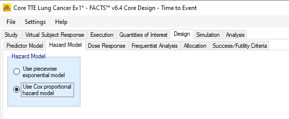
Second is the Piecewise exponential model. In this model, the observation period can be divided into separate time segments, and the hazard rate is estimated separately in each. When specifying the prior distributions for the hazard rates within time segments there are two different methods of specifying the prior - fixed priors or hierarchical priors. The time segments used in modeling the hazard rates can be different from those used in the specification of visits, VSRs, or dropout rates.
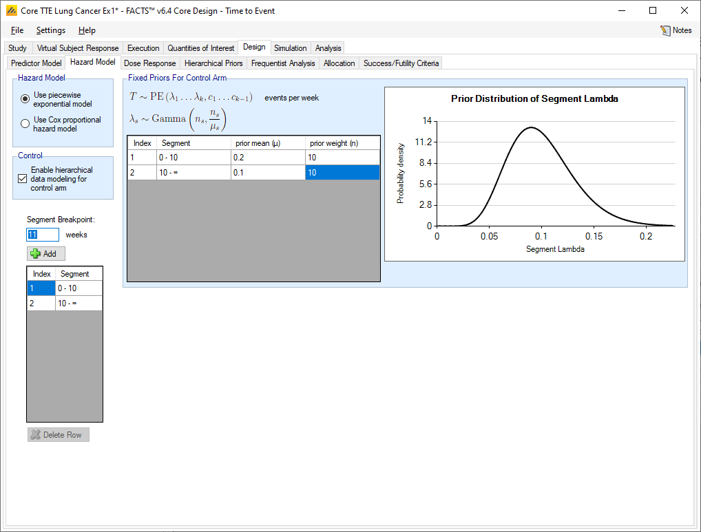
Fixed priors
If “Enable hierarchical data modeling for the control arm” is not selected, then independent gamma distributions with parameters specified in Hazard Rate tab’s table are used. The gamma parameters have been reparameterized so that the mean hazard rate and a weight (in terms of number of events) are provided instead of the traditional \(\alpha\) and \(\beta\) parameters.
Hierarchical Prior
If “Enable hierarchical data modeling for the control arm” is selected, then the independent priors specified per segment are augmented by additional data specified on the “Hierarchical Priors” tab.
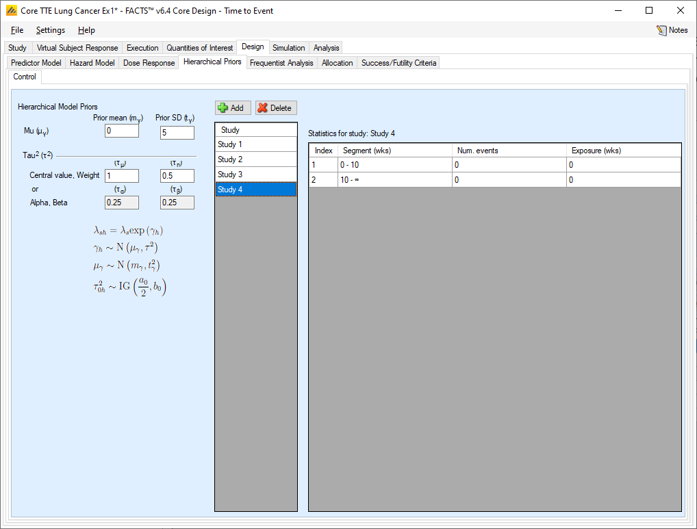
The additional data comes in the form of sufficient statistics from an outside data source. The sufficient statistics are, for each segment in each study, the number of events on the control arm and the control arm exposure time in subject weeks. The information from the prior study can be ‘down-weighted’ by reducing, pro-rata, the number of events and exposure time before entering them. By supplying the summary statistics from previous trials and specifying the parameters for prior distributions for the parameters of a hierarchical model, the gamma priors are updated and become the priors applied to the data collected on the virtual subjects.
The hyper-parameters are the mean and standard deviation of Normal distribution for the log hazard ratios of the event rates of the historical studies and the current study. The prior distribution for the mean hyper-parameter is a Normal distribution, for which the user specifies the mean and standard deviation. The prior distribution for the standard deviation hyper-parameter is an Inverse-Gamma distribution for which the user specifies either as a mean and a weight, or via Alpha and Beta parameters (depending on the user selection on Settings > Options > Gamma Distribution Parameters).
Unless the intent is to add information that is not included in the historic studies, the hyper parameters can and should be set so that they are ‘weak’ priors, centered on the expected values.
In this case the following would be reasonable:
Set the prior mean value for Mu as the mean of the log-hazard ratios of the event rates of the control arm and the historic studies (usually this will be 0)
Set the prior SD for Mu equal to at least the largest log hazard ratio of the event rates for the historic studies.
Set the mean for tau to the same value as the prior SD for Mu.
Set the weight for tau to be < 1.
One can traverse the spectrum from ‘complete pooling of data’ to ‘completely separate analyses’ through the prior for tau. If the weight of the prior for tau is small relative to the number of studies, then (unless set to a very extreme value) the mean of the prior for tau will have little impact and the degree of borrowing will depend on the observed data.
To give some prior preference towards pooling or separate analysis the weight for tau has to be large, relative to the number of historic studies. To have a design that is like pooling the historic studies, the mean for tau needs to be small – say 10% or less of the value suggested above. For there to be no borrowing from the historic studies the value for tau needs to be large – say 10x or more the value suggested above.
The best way to understand the impact of the priors is try different values and run simulations.