The Virtual Subject Response tab allows the user to explicitly define virtual subject response profiles, and/or to import virtual subject response from externally simulated PK/PD data. When simulations are executed, they will be executed for each profile specified by the user.
Explicitly Defined
Group Response
Response profiles may be added, deleted, and renamed using the table and corresponding buttons on the left hand side of the screen in Figure 1 Response rate values are entered for the treatment and control arms (if present) for each group directly into the Treatment Response Rate and Control Response Rate columns of the table. The graphical representation of these values updates accordingly.
In addition it is possible for the user to specify if a group “Should Succeed” using the “Should succeed” checkbox on each row. This is then used in the summary of the simulation results to compute how often the simulated trial was successful and groups that ‘Should Succeed’ were successful (reported in the column “Ppn Correct Groups”) and how often the simulated trial was successful and groups that were not marked ‘Should Succeed’ were successful (reported in the column “Ppn Incorrect Groups”).
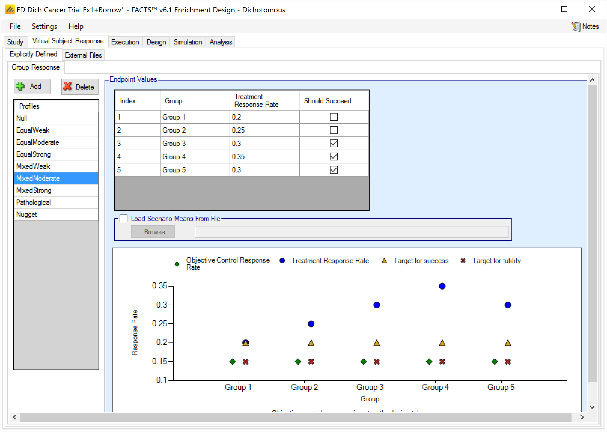
The graph that shows the response defined – as with all graphs in the application – may be easily copied using the ‘Copy Graph’ option in the context menu accessed by right-clicking on the graph. The user is given the option to copy the graph to their clipboard (for easy pasting into other applications, such as Microsoft Word or PowerPoint), or to save the graph as an image file.
Load Scenario Responses From File
If the “Load scenario means from a file” option is selected then in scenarios using this profile the simulations will use a range of dose responses.
Each individual simulation uses one set of responses from the supplied file, each row being used in an equal number of simulations. The summary results are thus averaged over all the VSRs in the file. The use of this form of simulation is somewhat different from simulations using a single rate or single external virtual subject response file. When all the simulations are simulated from a single version of the ‘truth’ then the purpose of the simulations is to analyse the performance of the design under that specific circumstance. When the simulations are based on a range of ‘truths’ loaded from an ‘.mvsr’ file then the summary results show the expected probability of the different outcomes for the trial over that range of possible circumstances. Note that to give different VSRs different weights of expectation, the more likely VSRs should be repeated within the file.
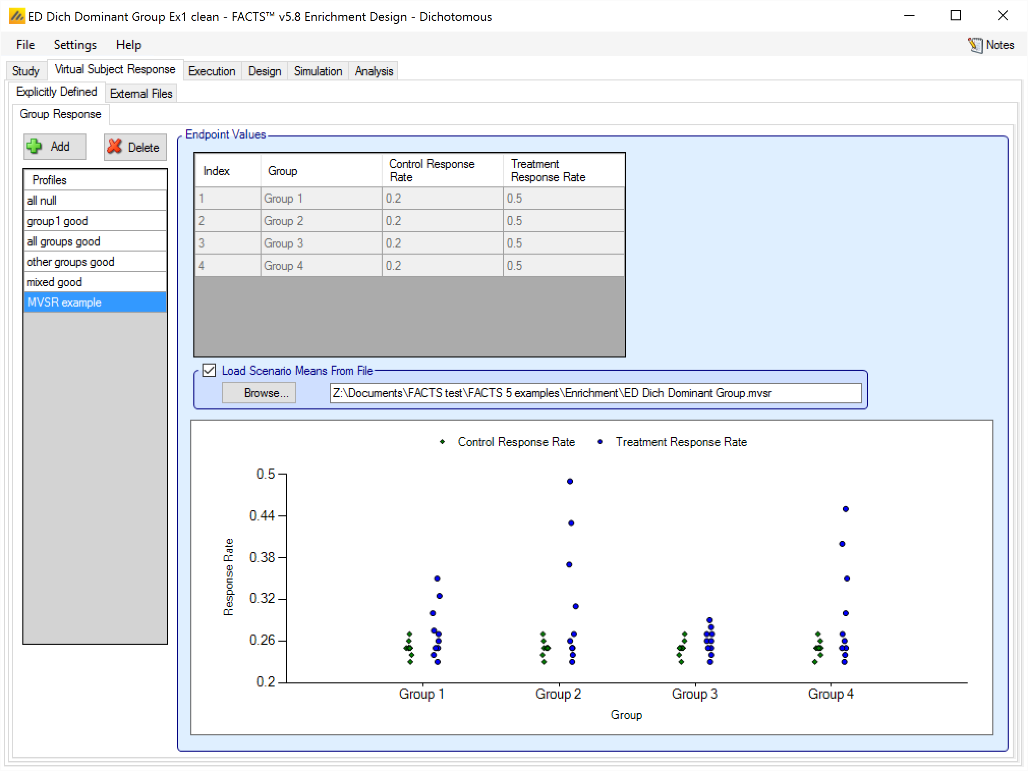
After selecting the “.mvsr” file the graph shows the individual mean responses and the overall mean response over all the VSRs.
The format of the file is a simple CSV text file. Lines starting with a ‘#’ character are ignored so the file can include comment and header lines. In the normal case the format is:
If a control arm is being used: Each line should contain columns [PT1, PT2, … , PTG, PCG, PC1, PC2, … , PCG] giving the true mean response probabilities (PTi) for the Treatment arm in each of the G groups, followed by the analogous parameters for the Control arms.
Without a control arm, using Objective Control: Each line should contain columns [PT1, PT2, … , PTG] giving the true mean response probabilities (PTi) for the Treatment arm in each of the G groups.
When using the Restricted Markov Model the format is:
If a control arm is being used: Each line should contain columns [P1T1, P1T2, … , P1TG, P0T1, P0T2, … , P0TG, P1C1, P1C2, … , P1CG, P0C1, P0C2, … , P0CG] giving the true mean response probabilities (P1Ti) and true mean non-response probabilities (P0Ti) for the Treatment arm in each of the G groups, followed by the analogous parameters for the Control arms.
Without a control arm, using Objective Control: Each line should contain columns [P1T1, P1T2, … , P1TG, P0T1, P0T2, … , P0TG] giving the true mean response probabilities (P1Ti) and true mean non-response probabilities (P0Ti) for the Treatment arm in each of the G groups.
For example:
# Dichotomous, 4 groups with control
#T1 T2 T3 T4 C1 C2 C3 C4
# 5 null cases
0.23, 0.23, 0.23, 0.23, 0.23, 0.23, 0.23, 0.23
0.24, 0.24, 0.24, 0.24, 0.24, 0.24, 0.24, 0.24
0.25, 0.25, 0.25, 0.25, 0.25, 0.25, 0.25, 0.25
0.26, 0.26, 0.26, 0.26, 0.26, 0.26, 0.26, 0.26
0.27, 0.27, 0.27, 0.27, 0.27, 0.27, 0.27, 0.27
# 5 increasingly good
0.25, 0.25, 0.25, 0.25, 0.25, 0.25, 0.25, 0.25
0.275, 0.31, 0.26, 0.30, 0.25, 0.25, 0.25, 0.25
0.30, 0.37, 0.27, 0.35, 0.25, 0.25, 0.25, 0.25
0.325, 0.43, 0.28, 0.40, 0.25, 0.25, 0.25, 0.25
0.35, 0.49, 0.29, 0.45, 0.25, 0.25, 0.25, 0.25
Longitudinal Models
If ‘Use longitudinal modeling’ has been checked on the ‘Study Info’ tab, and explicitly defined group responses have been specified, then it will be necessary to specify how to simulate the subjects’ responses at intermediate visits. This is done by specifying a transition method that can be combined with any of the response profiles to generate the intermediate results for subjects on treatment or control in all the groups.
The methods are parameterized so that its inclusion does not affect the response rate of the final endpoint to be simulated, and they scale automatically to suit each group response profile.
Click here for an overview of longitudinal models for dichotomous endpoints in the FACTS Core engine.
Enter / Retain Method
The Enter/Retain method is parameterized by setting probabilities for transition from non-responder to responder, and for remaining a responder once observed for each visit.
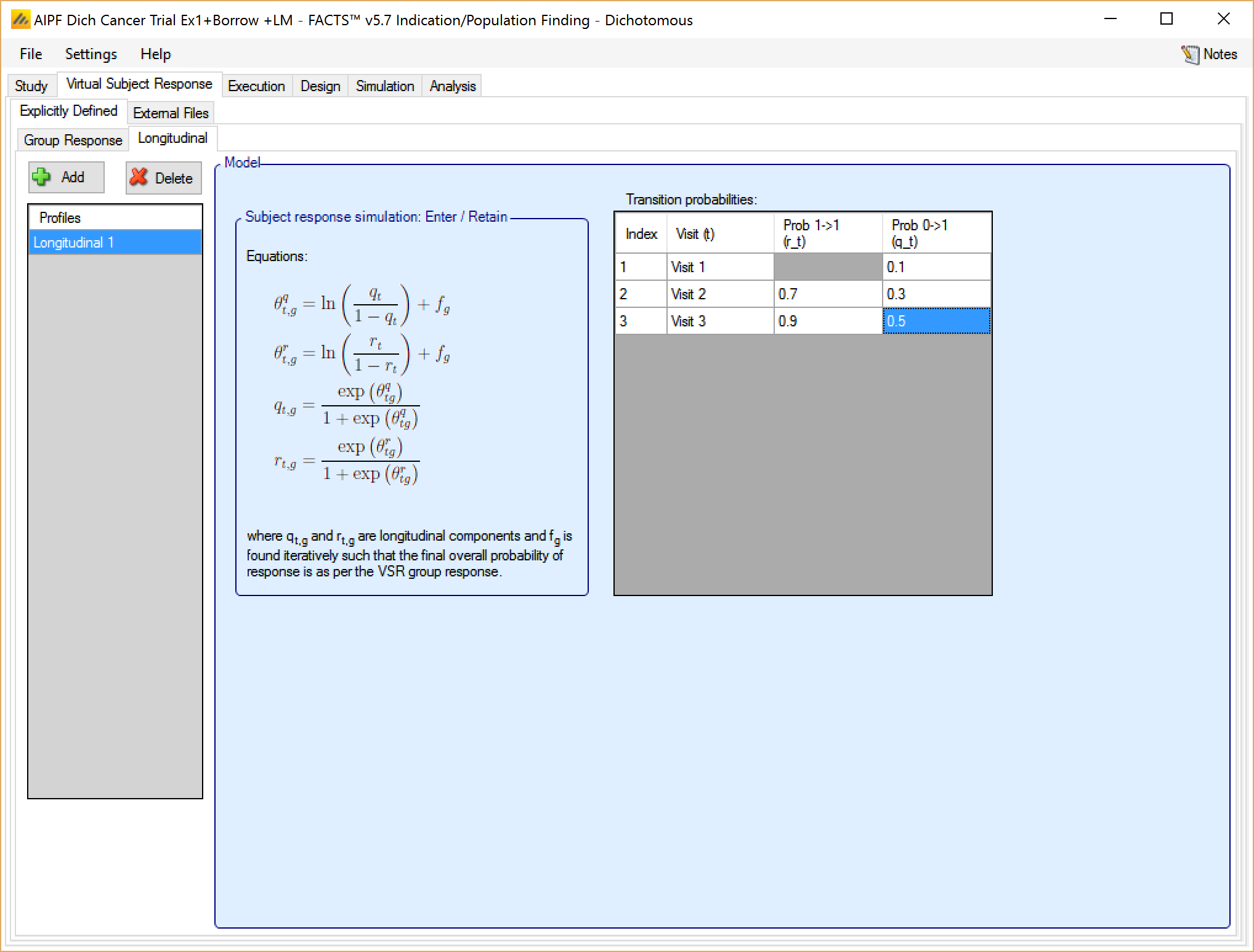
The transition probabilities will be modified for each treatment arm in each group response profile, to preserve the specified rate of response to simulate. This is done by finding (using numerical iteration) for each response rate to be simulated, the offset which, when added to the log odds of the all the transition probabilities, results in transition probabilities that give the required response rate.
Restricted Markov Model
If the restricted Markov model was selected on the Study Info tab, the subject simulation method is fully described by the overall probability of response and failure for each group.
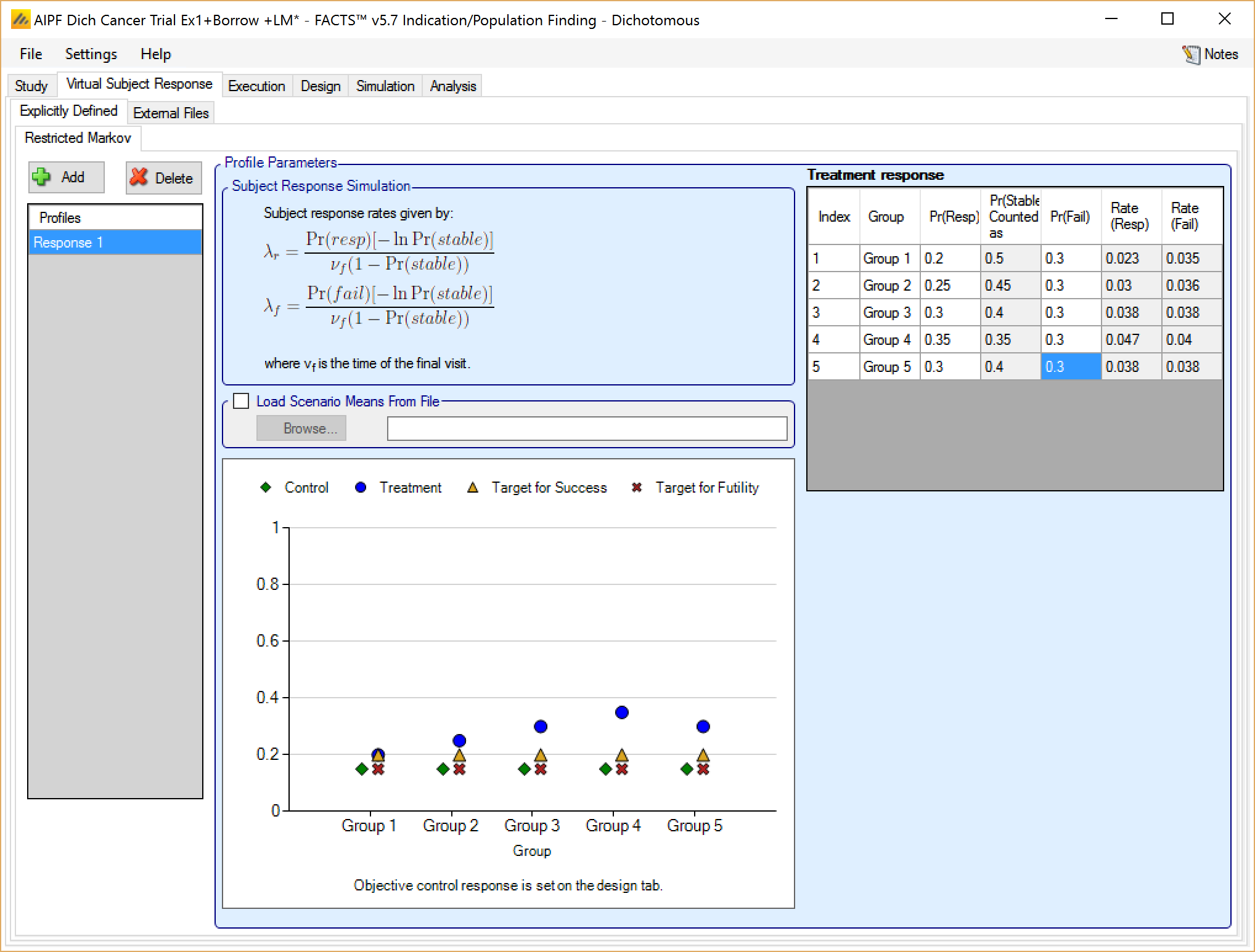
For each group, a final probability of response and failure are specified. The Probability of final stability is then inferred as the probability that neither response nor failure is observed. The response and failure rate can then be calculated as:
\[ \lambda_{r} = \frac{\Pr(resp)\left\lbrack - \ln{\Pr(stable)} \right\rbrack}{\nu_{T}\left( 1 - Pr(stable) \right)} \]
\[ \lambda_{f} = \frac{\Pr(fail)\left\lbrack - \ln{\Pr(stable)} \right\rbrack}{\nu_{T}\left( 1 - Pr(stable) \right)} \]
where \(\nu_{T}\) is the time of the final visit. When a virtual subject is recruited into the trial, a response and failure time are simulated based on the response and failure rates. If both events (response and failure) occur after the final visit, the simulated subject is counted as a final stability and their outcome is based on whether final stabilities count as success or failure as specified on the Study > Study Info tab. If one or both events occur before the final visit, the event that occurred first is taken as the subject’s final response because this is an absorbing state model. Once an outcome has been observed, that outcome remains for the rest of the treatment schedule.
If values are entered for the probability of response and failure that sum to greater than one, the probability of stability displays an error and the response rates are reported as NaN (not a number).
If values are entered for the probability of response and failure that sum to exactly one, the probability of stability is 0 and both response rates are effectively infinite. In this case, “**” is displayed as the response rate although these are valid settings.
External
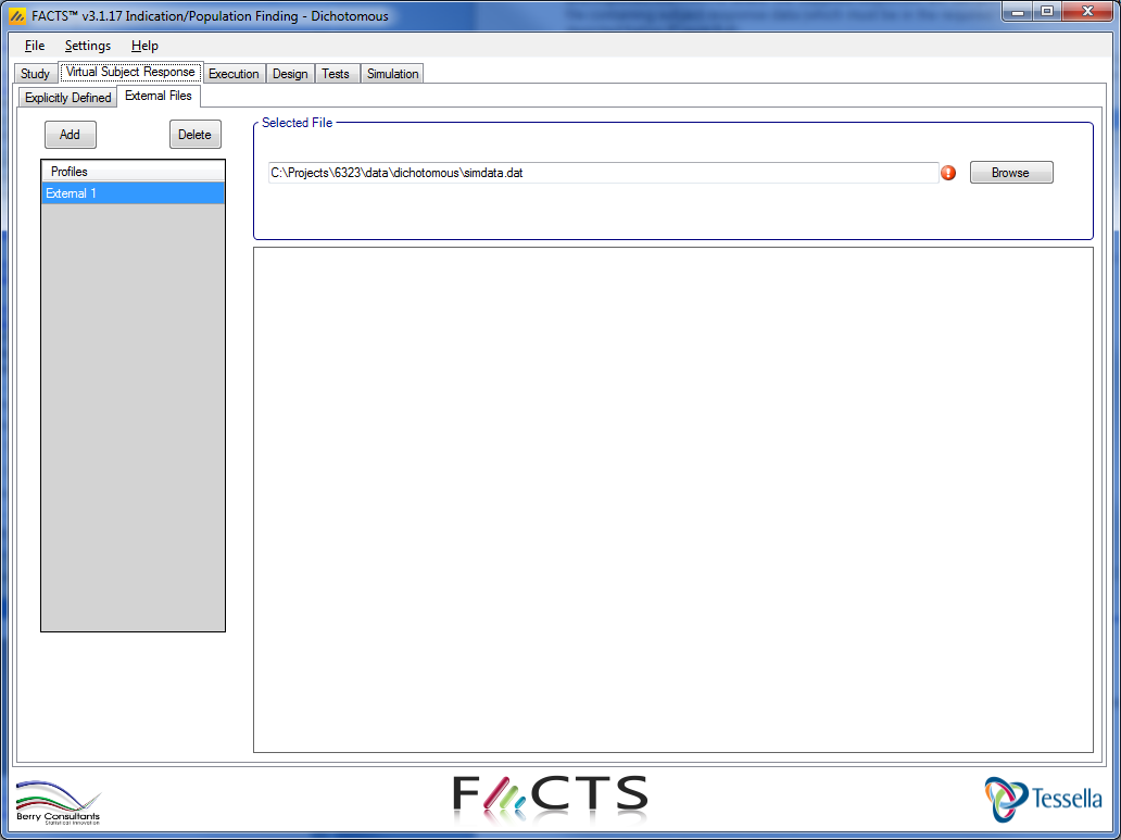
As well as simulating subject response within FACTS they can be simulated externally, from a PK-PD model for instance, and imported into FACTS, and the supplied responses are sampled from (with replacement) to provide the subject responses in the simulation. The specification of a file containing subject response data (which must be in the required format) can be done from the External Files sub-tab depicted below.
To import an external file, the user must first add a profile to the table. After adding the profile, a file selector window is opened and the user must select the file of externally simulated data. To change the selection, click the ‘Browse’ button.
Required Format of Externally Simulated Data
The supplied data should be in the following format: an ascii file with data in comma separated value format with the following columns:
Patient id (must be positive and change from subject to subject)
Group index (1, 2, 3,… )
Arm Index (1 = Control, 2 = Treatment)
Visit Id (1, 2, 3, …)
Response (0, 1), if the Restricted Markov model is being used then possible Response values are (0, 1, -1 = stable).
The GUI requires that the file name has a “.dat” suffix.
The following shows values from an example file. Note that all visits for each subject must be grouped together. Thus all the data for the first subject comes before that of the second, and so on.
#Patient ID, Group Index, Arm Index, Visit, Response
1, 1, 1, 1, 0
1, 1, 1, 2, 0
1, 1, 1, 3, 1
1, 1, 1, 4, 0
2, 1, 2, 1, 0
2, 1, 2, 2, 0
2, 1, 2, 3, 0
2, 1, 2, 4, 0
3, 2, 1, 1, 0
3, 2, 1, 2, 0
3, 2, 1, 3, 1
3, 2, 1, 4, 1
Simulated subjects will be drawn from this supplied list, with replacement, to provide the simulated response values.