Introduction
Purpose of this document
This document describes how use the Rule-Based Dose Escalation (DE) Simulator within FACTS (the Fixed and Adaptive Clinical Trial Simulator from now on referred to as Dose Escalation Fixed and Adaptive Clinical Trial Simulator Software). It is intended for all end users of the system.
Scope of this document
This document covers the Dose Escalation Fixed and Adaptive Clinical Trial Simulator Software by describing the user interface. It covers the 3+3, mTPI, mTPI-2, i3+3 and BOIN designs. It does not cover the CRM design engine which has its own User Guide. This document does also not address the internal workings of the design engines or algorithms, which are addressed in the associated Design Engine Specification.
The screenshots provided are specific to a particular installation and may not reflect the exact layout of the information seen by any particular user. They were taken from FACTS, 5 or later if changed, installed on Windows 7 and Windows 10. Different versions of Windows or the use of different Windows themes will introduce some differences in appearance. The contents of each tab, however, will be consistent with the software.
Citing FACTS
Please cite FACTS wherever applicable using this citation.
Definition of Terms
An overview of the acronyms and abbreviations used in this document can be found here.
FACTS Overview
The Fixed and Adaptive Clinical Trial Simulator allows designs for a clinical trial to be evaluated and compared to traditional designs, thus allowing designs to be optimized. The designs fit a selected model to endpoints of interest, and evaluate pre-specified decisions based on the properties of the fitted model. These decisions may include selecting the dose to allocate to the next subject, and whether sufficient data has been gathered to allow the trial to be stopped.
There are currently four non-deprecated design engines for Dose Escalation FACTS: “3+3”, mTPI, mTPI-2, i3+3, BOIN, CRM and 2D-CRM.
This User Guide covers “3+3”, mTPI, mTPI-2, i3+3 and BOIN. CRM and 2D-CRM have their own user guides.
The Rules Based Methods
The methods implemented are:
- BOIN (Yuan et al. 2016)
- mTPI (Ji et al. 2010)
- mTPI-2 (Guo et al. 2017)
- i3+3 (M. Liu, Wang, and Ji 2020)
- 3+3 (S. Liu, Cai, and Ning 2013)
See the papers for details, but a summary of the methods is given here.
All these methods start allocating at a given dose (currently in FACTS this is always the lowest dose), and allocate in cohorts of a fixed size (3+3 can only use cohorts of 3, the other methods allow a different cohort size to be specified). After each cohort they consider all the data on the dose just tested (but unlike the CRM not other doses) and decide whether to Escalate (“E), Stay (”S”) or De-Escalate (“D”).
In all these methods (except 3+3) the decisions are based on a specified target toxicity rate \(p_T\) and target interval around that rate (\(p_T \in [p_L, p_U]\), note that \(p_T\) need not be at the center of this interval). How they make that decision is the principal difference between the methods, and these are described in method specific sub-sections below.
All (except 3+3) share in the following:
If at the highest dose the decision is to Escalate, this is converted to Stay instead, if at the lowest dose the decision is to De-escalate, this is converted to Stay instead.
Using a Beta-binomial distribution based on the observed data (with a Beta(0.001, 0.001) prior) if the posterior probability that the toxicity rate exceeds the target rate with some probability (0.95 by default) then mark the dose as unacceptable and de-escalate (shown as “DU” in the decision tables). Stopping the trial if this is at the lowest dose.
At the end of the trial, MTD selection is after isotonic regression performed as follows:
Calculate the toxicity rate estimate at each dose (BOIN uses the observed rates, all others use the posterior mean toxicity, assuming a Beta(0.005, 0.005) prior and an independent Beta-Binomial model).
Impose monotonicity using isotonic regression (pool adjacent violators): where monotonicity is violated, the estimates of toxicity at the respective doses are replaced with their average.
We then select the dose with isotonically transformed toxicity rate estimate closest to the target toxicity rate.
If there is a tie, if the toxicity rate estimate is above the target toxicity rate then the lower dose is selected, if the toxicity rate estimate is below the target toxicity rate then the higher dose is selected.
mTPI
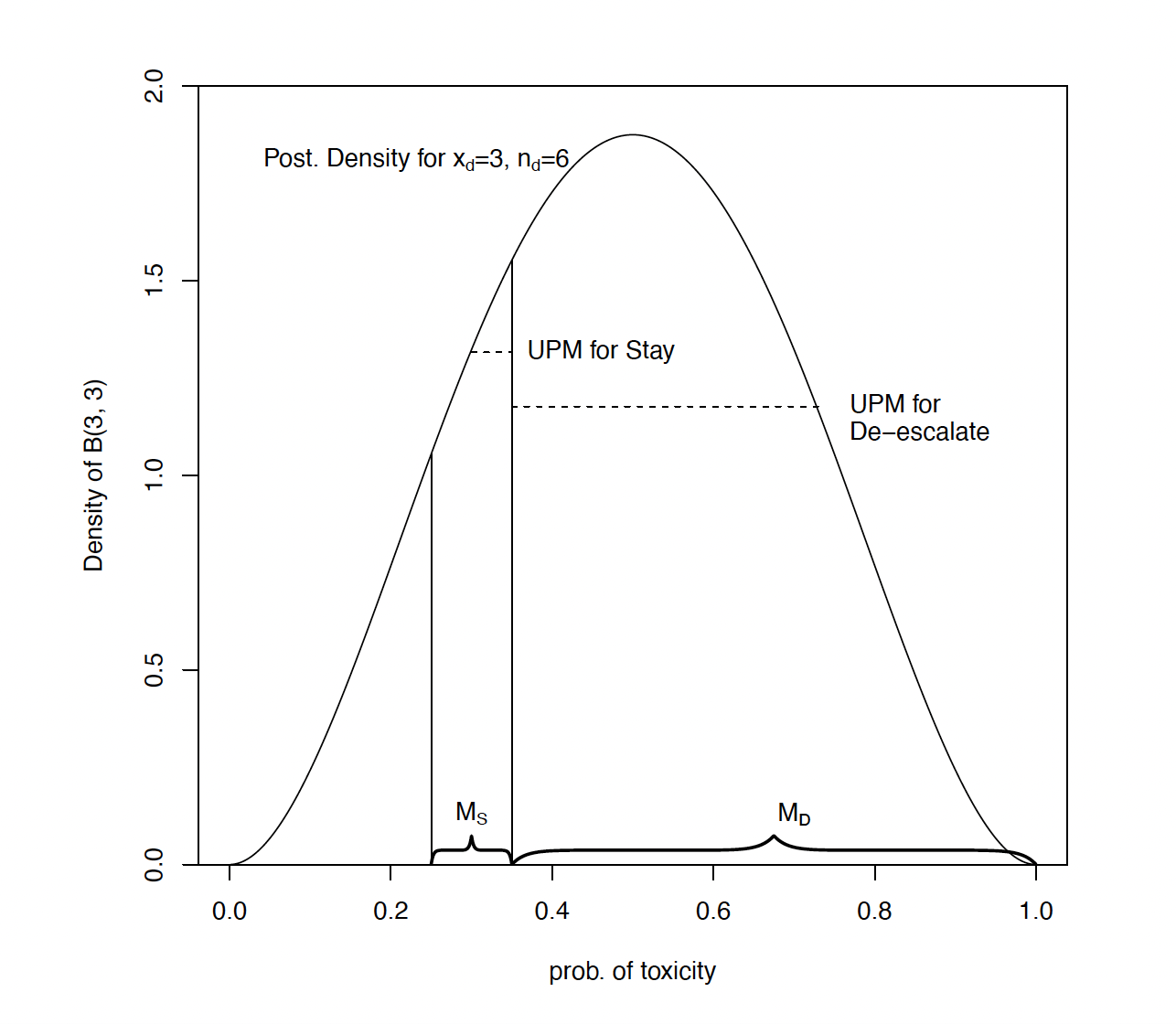
The E, S, D decision rule uses the Beta-Binomial distribution of the toxicity rate on a dose with a prior of Beta(0.001, 0.001). The Unit Probability Mass (UPM) is then calculated for three intervals: the interval below the target toxicity band, the interval corresponding to the target toxicity band and the interval above the target toxicity band. The UPM is the probability mass of the area divided by the length of the interval. The decision is then based on the interval with the highest UPM, E if its below the target toxicity band, S if it is the target toxicity band and D if its above the target toxicity band.
Below Figure 1 is taken from Guo et al. (2017). It shows the UPM in the target interval and above the target interval. It also illustrates what was perceived as a problem with the mTPI method, that gave rise to the development separately of mTPI-2, i3+3 and BOIN. With a target toxicity rate of 0.3 and target band of [0.25, 0.35], with 6 observations on a dose of which 3 had experienced a Dose Limiting Toxicity (DLT), the decision by the mTPI method is to Stay. It was generally considered that this was not safe decision.
mTPI-2
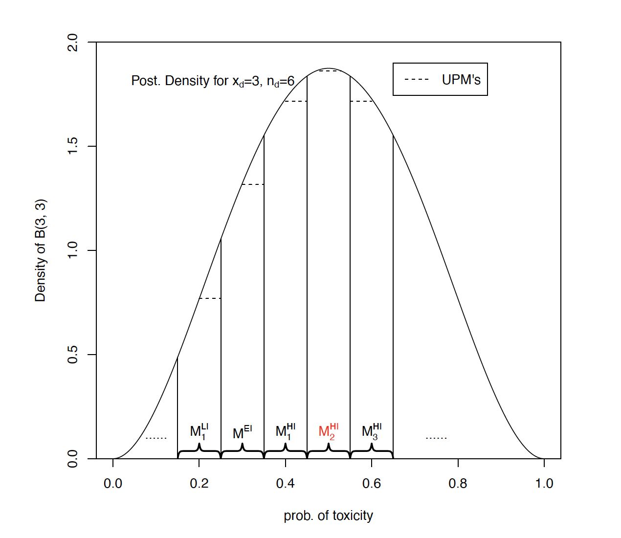
The E, S, D decision rule of mTPI-2 modifies that of mTPI by dividing the probability range into strips of equal width. The strips (with the possible exception of the first and the last whihc may need to be smaller) are the same width as the target toxicity band) and divide up the range above and below that band. The Unit Probability Mass (UPM) is then calculated for each of these strips and the strip with the highest UPM found. The decision is then based on the strip with the highest UPM, E if its below the target toxicity band, S if it is the target toxicity band and D if its above the target toxixcity band.
Below Figure 2 is taken from Guo et al. (2017). It shows the UPM for various strips with a target toxicity rate of 0.3 and target band of [0.25, 0.35], with 6 observations on a dose of which 3 had experienced a Dose Limiting Toxicity (DLT), the decision by the mTPI-2 method is to De-escalate.
i3+3
i3+3 bases its E, S, D decisions simply on the observed toxicity rate. If \(x\) is the number of observed toxicities at dose \(d\), and \(n\) the total number of observations, then
If \(\frac{x}{n}< p_L\), then escalated to the next dose (E).
Else if \(p_L < \frac{x}{n} < p_U\), then stay at this dose (S)
Else if \(p_U < \frac{x}{n}\), then
If \(\frac{x-1}{n} < p_L\), then stay at this dose (S).
Else, de-escalate (D).
BOIN
Based on the target Toxicity Band [\(p_L\), \(p_U\)], BOIN uses a formula to calculate the “optimal” boundaries \(\lambda_l\), \(\lambda_u\) to compare the observed toxicity rates to, which minimize incorrect (E, S, D) decisions: \[ \lambda_l = \frac{log \left(\frac{1-p_l}{{1-p_T}} \right)}{log\left(\frac{p_T(1-p)}{p_l(1-p_T)}\right)} \]
\[ \lambda_u = \frac{log \left(\frac{1-p_T}{{1-p_u}} \right)}{log\left(\frac{p_u(1-p_T)}{p_T(1-p_u)}\right)} \]
If \(x\) is the number of observed toxicities at dose \(d\), and \(n\) the total number of observations, then
If \(\frac{x}{n} < \lambda_l\) then escalate to the next dose (E).
Else if \(\lambda_l < \frac{x}{n} < \lambda_u\) then stay at this dose (S).
Else if \(\lambda_u < \frac{x}{n}\) then de-escalate (D).
The FACTS Rules-Based Dose Escalation GUI
The FACTS Rule-Based Dose Escalation GUI consists of five tabs:
The Study Tab for specifying the Treatment Arms (doses) available in the study.
The Virtual Subject Response tab for specifying response profiles to simulate. This is where a set of different toxicities rates per dose are specified that should represent the expected ‘space’ of the expected dose-toxicity profiles for the compound being tested.
The Design tab for specifying the dose escalation method (3+3/mTPI/mTPI-2/i3+3/BOIN), maximum number of cohorts and cohort size, cohort expansion (yes/no), target toxicity bounds and additional rules such as overdose control and stopping rules. These are the design choices open to the trial biostatistician. The expected consequences of these design choices are to be estimated by running simulations of the trials using the various virtual subject response profiles defined.
On the Simulation Tab, the user controls and runs simulations and can view the simulation results.
On the Analysis tab, the user can load an example data set and view the results of the FACTS analysis of that data using the current specified design.
Also on the menu bar, on the right hand side of the FACTS Window, is a button labeled “Notes”; clicking this button reveals a simple “notepad” window in which the user can maintain some simple notes that will be stored within the “.facts” file.
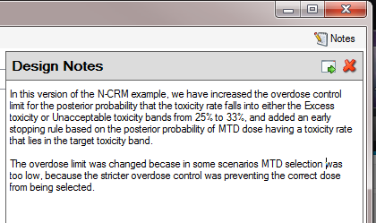
The notepad window comes with two further buttons: one to change the window to a free floating one that can be moved away from the FACTCS window; and the other to close it.
The Notes field can be used for any text the user wishes to store with the file. Suggested uses are: to record the changes made in a particular version of a design and why; and to comment on the simulation results. This will help when coming back to work that has been set aside, to recall what gave rise to the different version of a design.
Introduction
To open the application, select FACTS Dose Escalation from your Start menu. At different points in the FACTS GUI, the user is required to make decisions about how to model or simulate various aspects of a clinical trial. To simplify data entry, FACTS shows the user only the information that is relevant to the current decisions.
FACTS has a tabbed design to allow entry of different categories of information about the design.
The File menu allows the user to create a new design, open an existing design, save a design, or copy a design to a new name (Save as). The saved design includes all parameters entered as well as simulation results, if they have been produced.
The Settings menu provides the ability to configure how simulation jobs should be submitted to the Grid. Selecting whether to execute simulations locally or on the Grid is done from the Simulation tab.
The Help menu allows the user to learn more about the FACTS software and verify the application’s version number.
Finally, note that in all tabs of the application, red exclamation points

indicate errors in data entry from the user that must be corrected. Moving the cursor over the exclamation point causes a pop-up help text indicating what the error is, helping the user remedy the error.
Study
Treatment Arms
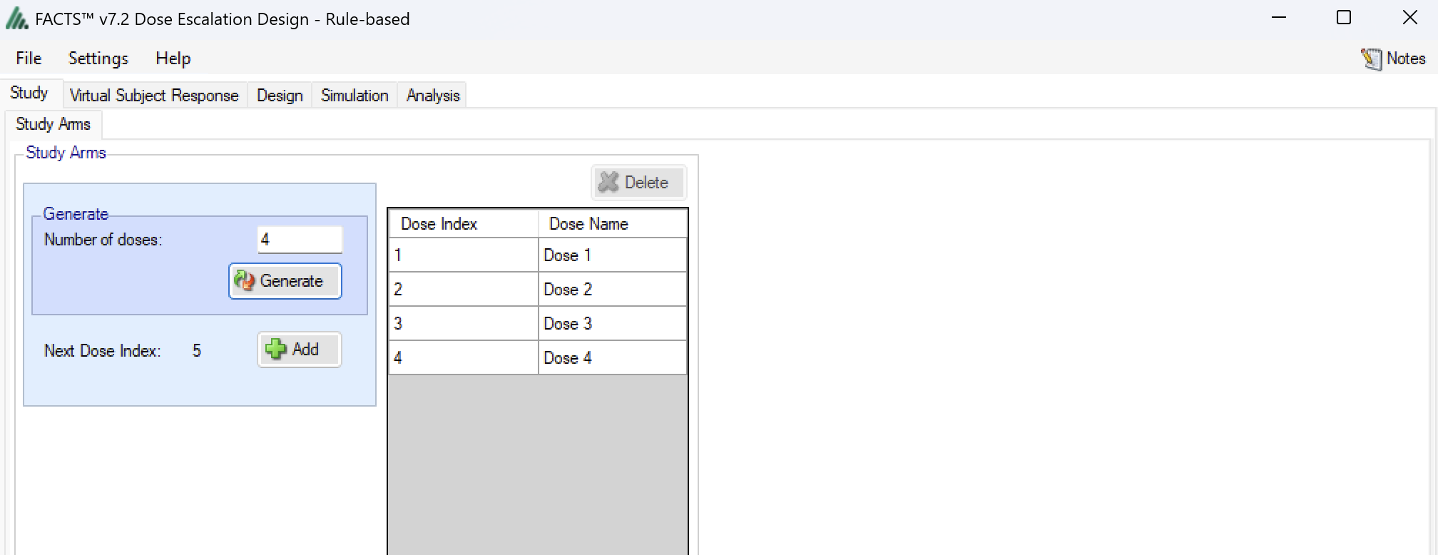
The Study > Treatment Arms tab (Figure 5) provides an interface for specifying the various dose levels available for use in the trial.
The user may add doses either explicitly or by auto-generation, as depicted below. The user may also edit the Dose Names within the table by double clicking on any existing dose name, however the index cannot be edited.
Virtual Subject Response
The Virtual Subject Response tab allows the user to explicitly define response profiles. When simulations are executed, they will be run separately for each profile defined by the user.
Explicitly Defined
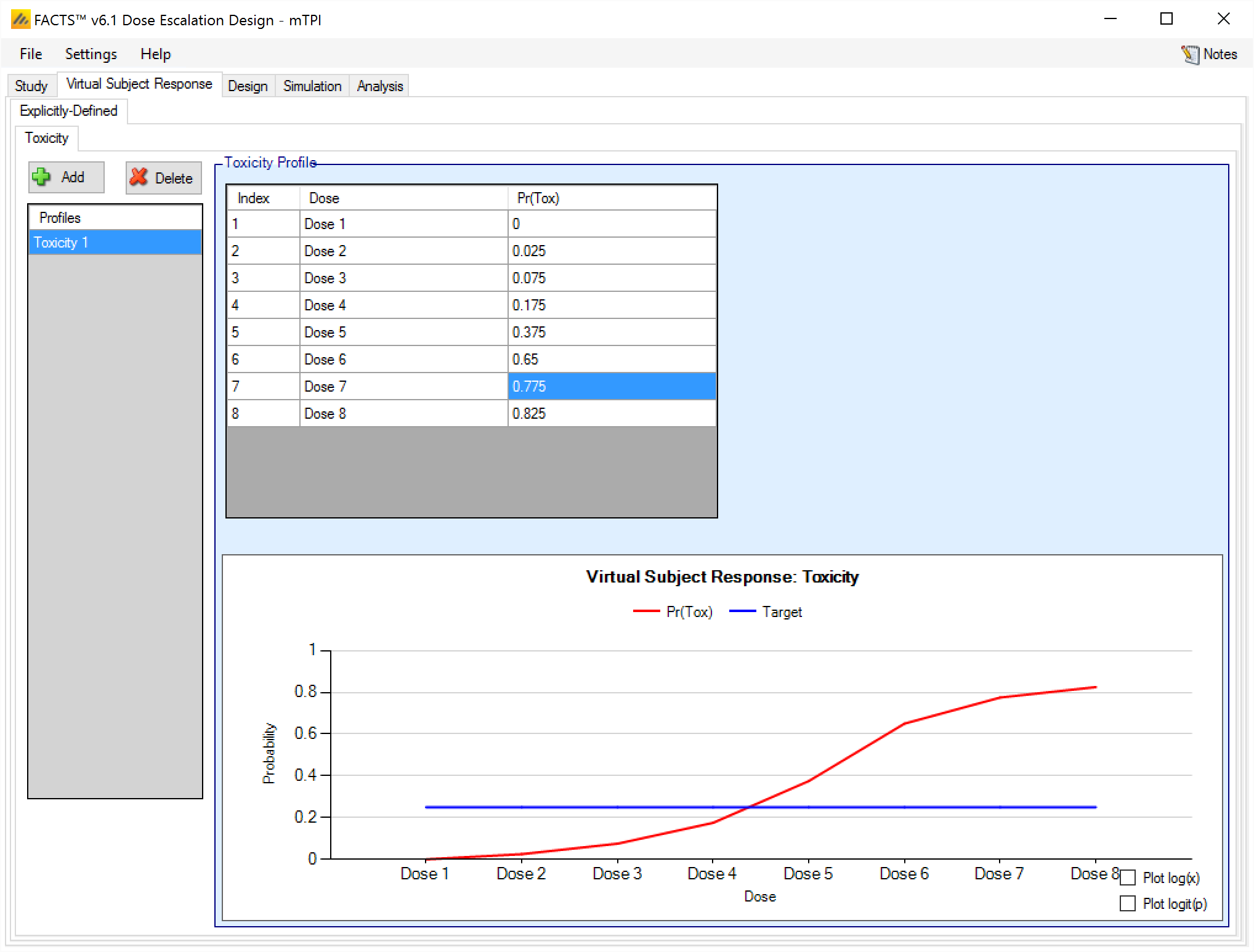
The Virtual Subject Response > Explicitly Defined > Toxicity sub-tab provides an interface for specifying one or more Toxicity profiles.
Toxicity profiles may be added, deleted, and renamed using the table and corresponding buttons on the left hand side of the screen in Figure 6. Toxicity values are entered directly into the Probability of Toxicity column of the table, and the graphical representation of these toxicity values updates accordingly. The graph may be modified by plotting the log of the dose strength as the x-axis, and by plotting the logit or the probability of toxicity as the y-axis.
This graph – as with all graphs in the application – may be easily copied using the ‘Copy Graph’ option in the context menu accessed by right-clicking on the graph. The user is given the option to copy the graph to their clipboard (for easy pasting into other applications, such as Microsoft Word or PowerPoint), or to save the graph as an image file.
Design
Options tab
The first option to choose in the Design > Options tab is the underlying algorithm to be used for the escalation, de-escalation and overdose rules. The choices are:
- BOIN (Yuan et al. 2016)
- mTPI (Ji et al. 2010)
- mTPI-2 (Guo et al. 2017)
- i3+3 (M. Liu, Wang, and Ji 2020)
- 3+3 (S. Liu, Cai, and Ning 2013)

Options that are common to all algorithms are:
- Max Number of Cohorts: This in conjunction with the cohort size gives the maximum sample size of the trial. After the selected number of cohorts have been included, no further cohorts will be included and the MTD will be selected according to the respective algorithm.
- Cohort Size: The number of trial participants included in each cohort. In 3+3, this defaults to “3” and cannot be changed. The maximum sample size of the trial is simply: Max Trial Size (cohorts) * Cohort Size.
- Cohort Expansion: The user can specify that after the dose escalation phase of the trial has completed, the simulation is to include an ‘expansion cohort’ (allocated at the final estimate of the MTD) and how large that expansion cohort will be.
The further options depend on the chosen design algorithm chosen. Please select the algorithm of interest to learn more. If you are interested in mTPI, mTPI-2, BOIN or i3+3, please select “Non 3+3” in the first stage.
Given all the options specified, the matrix of dosing decisions is displayed on the right hand side. This shows the dosing decision given the number of subject treated at the current dose and the number of toxicities observed:
E Escalate
S Stay
D De-escalate
DU De-escalate and do not revisit
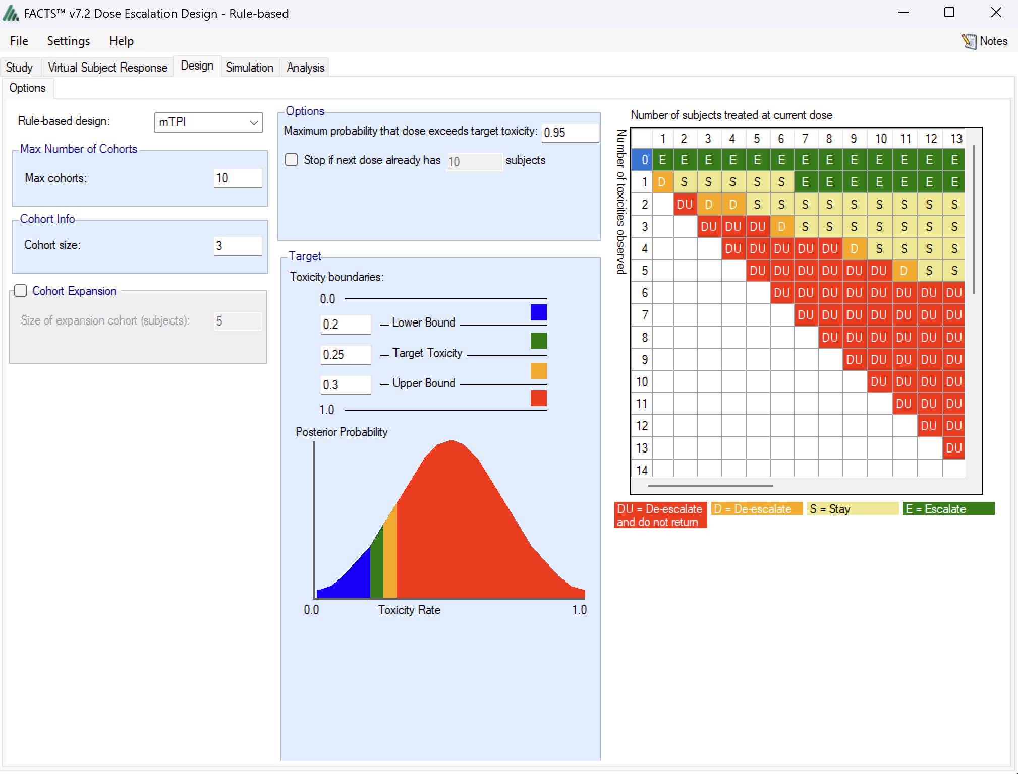
As an example, if the value of row 2, column 6 is “E”, the algorithm would want us to escalate to the next dose if we had observed 2 toxicities in 6 trial participants.
Additional options include:
Maximum probability that dose exceeds target toxicity: This is an option to prevent re-escalating to a dose (the “DU” or Do not Use category in the decision matrix) if the posterior probability (based on a Beta-Binomial model per dose) that the toxicity rate is above the target toxicity is greater than the selected value (0.95 is the default).
Stop if next dose already has X subjects: This is an option that allows an early stopping rule to be specified that if the dose to be allocated next already has the maximum number of subjects on it then it is declared the MTD. Setting this value shrinks the size of the decision matrix.
Target Toxicity boundaries: The user specifies target toxicity rate, as well as the lower and upper acceptable bounds on the toxicity rate, effectively creating four distinct buckets for doses:
- Underdosing: Doses with a toxicity rate falling into the [0,lower bound] bucket
- Target: Doses with a toxicity rate falling into the (lower bound,target] bucket
- Excess Toxicity: Doses with a toxicity rate falling into the (Target,upper bound] bucket
- Unacceptable Toxicity: Doses with a toxicity rate falling into the (Upper bound,1] bucket
These bounds are then used in the different algorithms to create the decision table.
BOIN has extra options compared to mTPI, mTPI-2 and i3+3:
- Use default BOIN bounds: Whether or not the lower and upper toxicity bound should be calculated automatically using the BOIN defaults (lower bound = 0.6*target, upper bound = 1.4*target), or whether they are chosen by the user.
- Stay when seeing 1/3 toxicities: Whether or not to overwrite the algorithm’s decision to stay at the current dose level when seeing 1 DLT in 3 trial participants. This is useful to mimic the behavior of 3+3 which is often expected by clinicians.
- De-escalate when seeing 2/6 toxicities: Whether or not to overwrite the algorithm’s decision to de-escalate from the current dose level when seeing 2 DLTs in 6 trial participants. This is useful to mimic the behavior of 3+3 which is often expected by clinicians.
- Initial dose index: The user may specify the dose level that the first cohort will be allocated to. Might be useful in cases where we believe there is a (small) chance the initial cohort will experience DLTs. In a real world situation, observing too many DLTs on the first dose level likely terminates the study, whereas if we had started at dose level 2, we have a fall back dose level to de-escalate to.
- Include final validation cohort: Whether to include an additional cohort at the chosen MTD after the original 3+3 algorithm has terminated.
Simulation
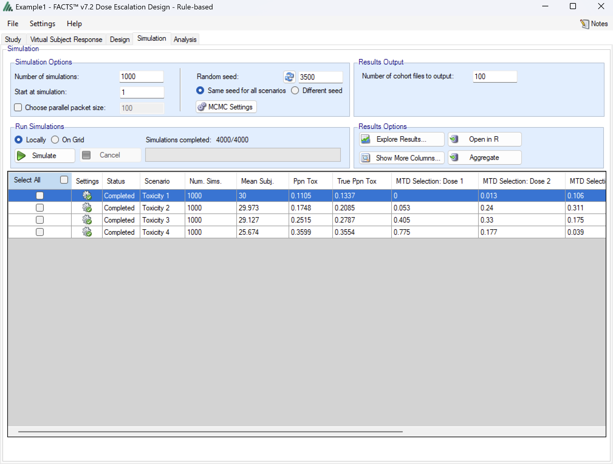
The Simulation tab allows the user to execute simulations for each of the scenarios specified for the study. The user may choose the number of simulations, whether to execute locally or on the Grid, and modify the random number seeds (Figure 9).
If completed results are available, the actual number of simulations run for each scenario is reported in one of the first columns of the results table. The value displayed in the “Number of Simulations” control is the number of simulations that will be run if the user clicks on the ‘Simulate’ button.
FACTS uses Markov Chain Monte Carlo methods in the generation of simulated patient response data and trial results. In order to exactly reproduce a statistical set of results, it is necessary to start the Markov Chain from an identical “Random Seed”. The initial random seed for FACTS simulations is set from the simulation tab, the first thing that FACTS does is to draw the random number seeds to use at the start of each simulation. It is possible to re-run a specific simulation, for example to have more detailed output files generated, by specifying ‘start at simulation’.
Say the 999th simulation out of a set displayed some unusual behavior, in order to understand why, one might want to see the individual interim analyses for that simulation (the “weeks” file), the sampled subject results for that simulation (the “Subjects” files) and possibly even the MCMC samples from the analyses in that simulation. You can save the .facts file with a slightly different name (to preserve the existing simulation results), then run 1 simulation of the specific scenario, specifying that the simulations start at simulation 999 and that at least 1 weeks file, 1 subjects file and the MCMC samples file (see the “MCMC settings” dialog) are output.
Even a small change in the random seed will produce different simulation results.
The same random number seed is used at the start of the simulation of each scenario. If two identical scenarios are specified then identical simulation results will be obtained. The same may happen if scenarios or designs only differ in ways that have no impact on the trials being simulated, for instance designs that have no adaptation, or scenarios that don’t trigger any adaptation (e.g. none of the simulations stop early).
The user can specify:
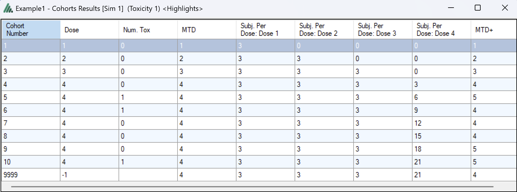
the number of simulations for which ‘Cohorts’ files are written. ‘Cohorts’ files record the data, analysis and recommendation at each interim (after each cohort).
The parallelization packet size, this allows simulation jobs to be split into runs of no-more than the specified number of trials to simulate. If more simulations of a scenario are requested than can be done in one packet, the simulations are started as the requisite number of packets and the results combined and summarized when they are all complete – so the final results files look just as though all the simulations were run as one job or packet. When running simulations on the local machine FACTS enterprise version will process as many packets in parallel as there are execution threads on the local machine. The overhead of packetisation is quite low so a packet size of 10 to 100 can help speed up the overall simulation process – threads used to simulate scenarios that finish quicker can pick up packets for scenarios that take longer, if the number of scenarios is no directly divisible by the number of threads packetisation uses all threads until the last few packets have to be run and finally the “Simulations complete” figure can be updated at the end of each packet, so the small the packet the better FACTS can report the overall progress.
To run simulations
Click in the check box in each of the rows corresponding the to the scenarios to be run. FACTS displays a row for each possible combination of the ‘profiles’ that have been specified: - baseline response, dose response, longitudinal response, accrual rate and dropout rate. Or simply click on “Select All”.
Then click on the “Simulate” button.
During simulation, the user may not modify any parameters on any other tab of the application. This safeguard ensures that the simulation results reflect the parameters specified in the user interface.
When simulations are started, FACTS saves all the study parameters, and when the simulations are complete all the simulation results are saved in results files in a “_results” folder in the same directory as the “.facts” file. Within the “_results” folder there will be a sub-folder that holds the results for each scenario.
How many simulations to run?
After first entering a design it is worth running just a small number of simulations such as 10 to check that the scenarios and design have been entered correctly. If all 10 simulations of a ‘null’ scenario are successful, or all 10 simulations of what was intended to be an effective drug scenario are futile, it is likely there has been a mistake or misunderstanding in the specification of the scenarios or the final evaluation or early stopping criteria.
Once the design and scenarios look broadly correct, it is usually worth quickly collecting rough estimates of the operating characteristics using around 100 simulations for each scenario. 100 simulations is enough to spot designs having very poor operating characteristics such as very high type-1 error, very poor power, a strong tendency to stop early for the wrong reason, or poor probability of selecting the correct target. 100 simulations is also usually sufficient to spot problems with the data analysis such as poor model fits and significant bias in the posterior estimates.
Typically 1,000 simulations of each scenario of interest is required to get estimates of the operating characteristics precise enough to compare designs and tune the parameters. (Very roughly rates of 5% (such as type-1 error) can be estimated to about +/-1.5% and rates of around 80% (such as power) estimated +/- 2.5%)
Finally around 10,000 simulations of the scenarios of interest is required to give confidence in operating characteristics of a design and possibly to select between the final shortlisted designs (Approximately rates of 5% can be estimated to about +/-0.5% and rates of around 80% estimated +/- 1%).
There may be many operating characteristics need to be compared over a number of scenarios, such as expected sample size, type-1 error, power, probability of selecting a good dose as the target and quality of estimation of the dose-response.
However frequently these will be compared over a range of scenarios, it may not be necessary to run very large number of simulations for each scenario if a design shows a consistent advantage on the key operating characteristics over the majority of the scenarios.
Simulation results
In the main screen the summary results that are usually of principal interest are displayed, the results summarised by scenario.
Show more columns: Allows the user to open additional windows on the simulation results, the windows available are:
All: A window containing all the summary results columns
Highlights: (all) a separate window with the results shown on the main tab
Allocation, Observed: (all) summary results of the number of subjects allocated, the number allocated to each dose, the number of toxicities observed and the number of toxicities observed per dose
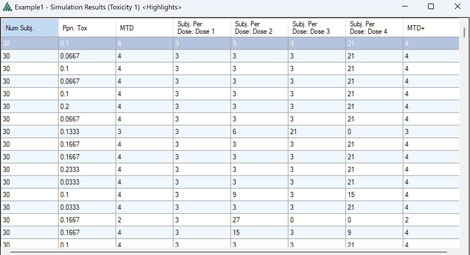
Simulation Results: a window displaying the individual simulation results for each simulation of the currently selected scenario
Explore Results: opens the FACTS built in options for visualizing the results for both the currently selected scenario and across all scenarios. See Section 11 below for a description of the graphs.
Aggregate: opens a control that allows the user create aggregated results files from all the scenarios. The user can select which scenarios to include, and whether the results should be pivoted by dose. The resulting files are stored in the simulation results folder.
Open in R: If aggregated files have been created then clicking this button on the simulations tab will open control that allows the user to select which aggregations to load into data frames as R is opened. Otherwise it will offer to open R using the files in the currently selected scenario.
Right Click Menu: right clicking the mouse on a row of results in the simulation tab brings up a ‘local’ menu of options:
Open results folder: Opens a file browser in the results folder of the scenario, allowing swift access to any of the results files.
Simulation results: Opens a window displaying the individual simulation results for each simulation of the currently selected scenario
Open in R: opens a control that will launch R, first loading the selected files in the results folder as data frames.
View Graphs: launches the graph viewer to view the results of the currently selected scenario.
MCMC Settings
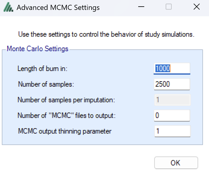
The first two values specify two standard MCMC parameters –
The length of burn-in is the number of the initial iterations whose results are discarded, to allow the sampled values to settle down.
The number of samples is the number of subsequent iterations whose results are recorded in order to give posterior estimates of the values of interest (in this case α and β).
If the Number of MCMC samples to output value is set to N, where N > 0, then all the sampled values at each interim in the first N simulations are output, allowing the user to check convergence.
The MCMC output thinning parameter can be used to reduce the amount of data output to the MCMC file. It does not reduce the amount of MCMC samples used within the model fitting.
To obtain the MCMC sampled values for a particular simulation, keep the same Random number seed and use Start at simulation to specify the simulation in question and run just 1 simulation.
FACTS Grid Simulation Settings
If you have access to a computational grid, you may choose to have your simulations run on the grid instead of running them locally. This frees your computer from the computationally intensive task of simulating so you can continue other work or even shutdown your PC or laptop. In order to run simulations on the grid, it must first be configured, this is normally done via a configuration file supplied with the FACTS installation by the IT group responsible for the FACTS installation.
Detailed Simulation Results
After simulation has completed and simulation results have been loaded, the user may examine detailed results for any scenario with simulation data in the table by double-clicking on the row. A separate window (as in Figure 11) will reveal more detailed results about the simulation.
Right-clicking on a row displays a context menu from which the user can also view the corresponding cohort results:
Aggregation
Aggregation combines the csv output from multiple scenarios into fewer csv files. The Aggregate… button displays a dialog which allows the user to select what to aggregate.
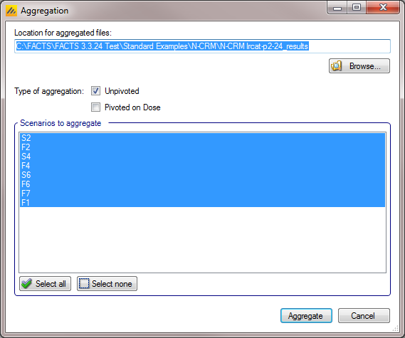
The default location for the aggregated files is the results directory for the study, but this can be changed.
Aggregation may be performed with or without pivoting on group, or both.
Unpivoted files will have one row for each row in the original files.
In pivoted files each original row will be split into one row per dose, plus two extra rows for ‘below lowest’ and ‘above highest’.
Where there is a group of columns for each dose, they will be turned into a single column with each value on a new row.
If there is no value for the below lowest or above highest rows, they will be left blank.
Values in columns that are independent of group will be repeated on each row.
The default is to aggregate all scenarios, but any combination may be selected.
Pressing “Aggregate” generates the aggregated files.
Each type of csv file is aggregated into a separate csv file whose name begins agg_ or agg_pivot_, so agg_summary.csv will contain the rows from each of the summary.csv files, unpivoted. cohortsNNN.csv files are aggregated into a single agg_[pivot_]cohorts.csv file. Doses.csv is identical for all scenarios and so is not aggregated.
Each aggregated file begins with the following extra columns, followed by the columns from the original csv file:
| Column Name | Comments |
|---|---|
| Scenario ID | Index of the scenario |
| Toxicity Profile | A series of columns containing the names of the various profiles used to construct the scenario. Columns that are never used are omitted. |
| Agg Timestamp | Date and time when aggregation was performed |
| Sim | Simulation number. Only present in the cohorts file. |
| Dose | Only present if pivoted |
The Summary Results Columns
Highlights (All)
These are the columns displayed on the simulations tab after simulations are completed, the can also be displayed in the separate “Highlights” results window.
| Column Title | Number of columns | Engines | Description |
|---|---|---|---|
| Select | 1 | All | Not an output column, this column contains check box to allow the user to select which scenario to simulate. The ‘Select All’ button causes them all to be checked. |
| Status | 1 | All | This column reports on the current status of simulations: Completed, Running, No Results, Out of date, Error. It is updated automatically. |
| Scenario | 1 | All | This gives the name of the scenario. In the N-CRM this is simply the name of the Toxicity response profile to be simulated (in other Design Engines the scenario may be a combination of a number of profiles). |
| Num Sims | 1 | All | The number of simulations that were run to produce the displayed results. |
| Random Number Seed | 1 | All | Base random number seed used to perform the simulations. |
| Mean Subj. | 1 | All | This is the mean (over the simulations) of the number of subjects recruited in this scenario. |
| PPn. Tox | 1 | All | This is the average proportion of the subjects recruited that experienced a toxicity in the simulations of this scenario. |
| SD Ppn. Tox | 1 | All | This is the standard deviation of the proportion of toxicity across the simulations of this scenario. |
| True Ppn Tox | 1 | All | This is the average true probability of toxicity over the simulations. The ‘true probability of toxicity’ in a simulated trial is the average of the probabilities of toxicity all the subjects are exposed to, given the toxicity response profile of the scenario. |
| MTD Selection: <dose> | One per dose | All | For each dose, this is proportion of the simulations where it was selected as the MTD (Maximum Tolerated Dose) at the end of the study. The dose chosen will be the dose with the highest posterior probability being the MTD (closest dose to having the target toxicity rate – or “nearest below” or “nearest above” as selected by the user on the Study Info tab. |
| Ppn(All Tox) | 1 | All | The proportion of the simulations that stopped because all doses were too toxic. |
| Ppn(Early Success) | 1 | All | The proportion of the simulations that stopped because sufficient stopping rules were met before the maximum number of cohorts had been treated. |
| Ppn(Cap) | 1 | All | The proportion of the simulations that stopped because the maximum number of cohorts had been treated. |
Allocations, Observed
| Column Title | Number of columns | Engines | Description |
|---|---|---|---|
| Scenario | 1 | All | This gives the name of the scenario. In the N-CRM this is simply the name of the Toxicity response profile to be simulated (in other Design Engines the scenario may be a combination of a number of profiles). |
| Mean Subj. | 1 | All | This is the mean (over the simulations) of the number of subjects recruited in this scenario. |
| Ppn. Tox | 1 | All | This is the average proportion of the subjects recruited that experienced a toxicity in this scenario. |
| SD PPn. Tox | 1 | All | This is the standard deviation of the proportion of toxicity across the simulations, |
| True Ppn Tox | 1 | All | This is the average true probability of toxicity over the simulations. The ‘true probability of toxicity’ in a simulated trial is the average of the probabilities of toxicity all the subjects are exposed to, given the toxicity response profile of the scenario. |
| Subj. Per Dose: <dose> | One per dose | All | This is the mean (over the simulations) of the number of subjects assigned to each dose. |
| SD Subjects: <dose> | One per dose | All | This is the standard deviation of the number of subjects assigned to each dose across the simulations. |
| Tox. Per Dose: <dose> | One per dose | All | This is the mean (over the simulations) of the number of toxicities observed at each dose. |
| SD Tox. Per Dose: <dose> | One per dose | All | This is the standard deviation of the number of toxicities observed at each dose across the simulations. |
| 80% Num Subj | 1 | All | This is the 80th centile of the overall number of subjects recruited in each simulation. |
Graphs of Simulation Results
The ‘View Graph’ button on the simulation tab also allows the user to view Summary graphs for the currently selected row of data in the summary results table. A separate Summary Graphs window will appear. The types of graphs available for viewing are listed in the left-hand side of the window; clicking on a graph type displays that graph. Note that some graphs will not be available if they are not relevant to the type of design the user has simulated. By right clicking on the graph the user can access the context menu that allows a copy of the graph to be copied to the Windows’ clipboard or saved as an image (‘.png’) file.
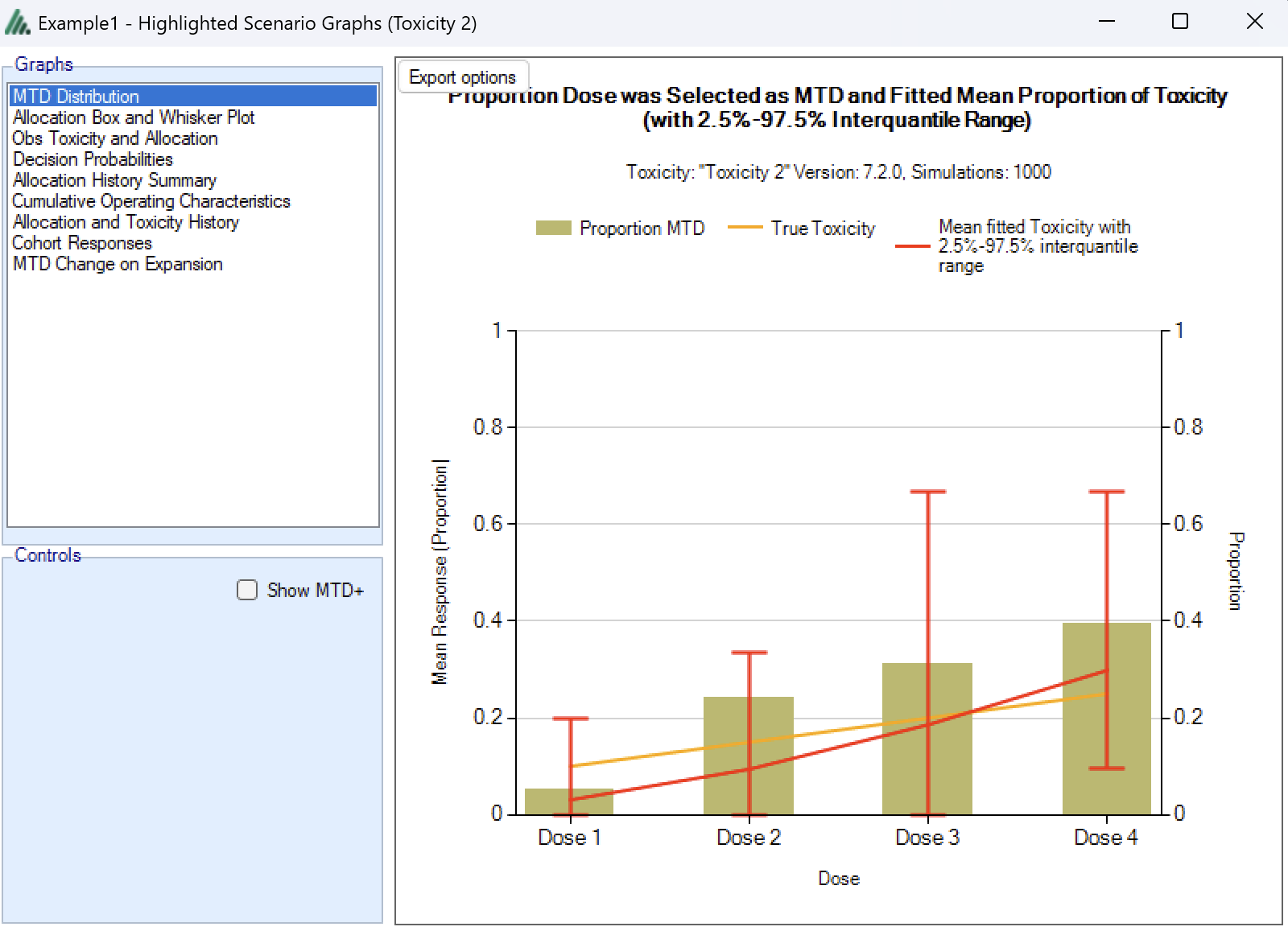
MTD Distribution
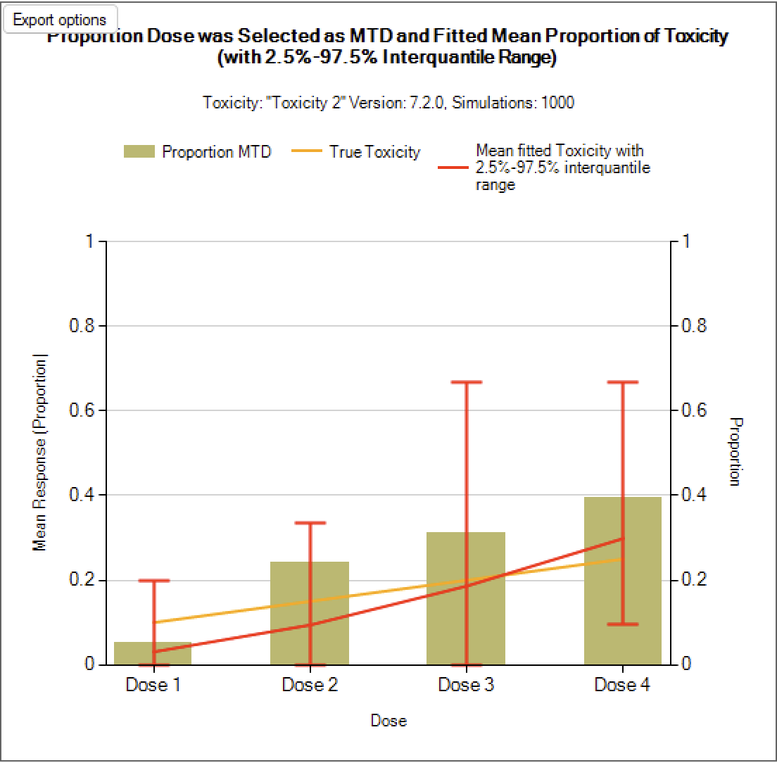
These graphs show the proportion of times each dose has been selected as a particular target dose as a brown bar, along with lines showing the mean fitted toxicity and the simulated ‘true’ toxicity. The ‘error’ bars on the mean estimated toxicity are the 95% interval of the mean estimates across the simulations.
Allocation Box and Whisker plot
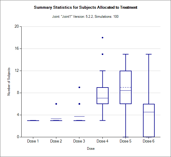
This graph displays a box and whisker plot of the number of subjects allocated to each dose over the simulations. These plots show:
The mean allocation over all simulations at each dose plotted as a solid line.
The median value is plotted as a dashed line.
The 25-75th quantile range is plotted as the “box” portion of each point.
The “whiskers” extend to the largest and smallest values within 1 ½ times the interquartile range from either end of the box.
Points outside the whisker range are considered outliers, and are plotted as small blue dots. Note that it may be difficult to see all of these symbols if they are plotted at the same value.
Obs Tox and Alloc / Toxicity and Allocation
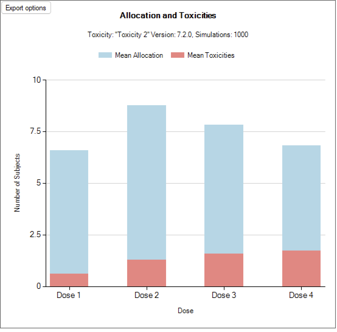
These graph show the mean allocation to each dose and the mean number of toxicities observed at each dose.
Simulation Allocation History
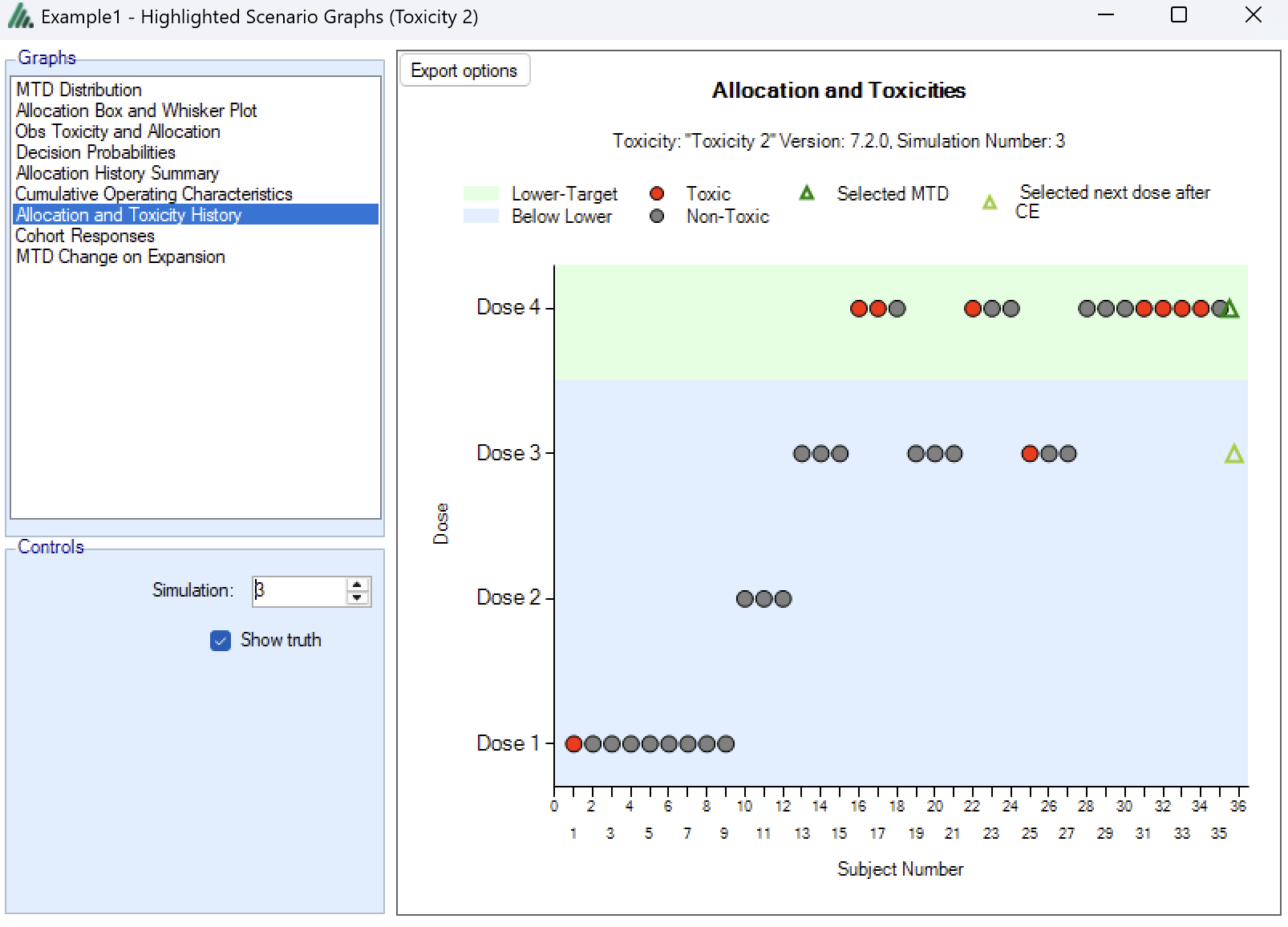
This graph shows the allocation and toxicity history for an individual simulation. Each dot represents a subject, the dot is colored red if toxicity was observed, and grey otherwise. The subjects’ outcomes are displayed left to right in the order in which they were dosed, and at a height corresponding to the dose they were given.
The graph also indicates the selected MTD based on all the data (and given the algorithm that was chosen). In case an expansion cohort was included, a separate symbol marks the dose that the algorithm would assign patients to had the trial not stopped at that particular sample size (this is in some way a marker to investigate whether the expansion cohort has changed our beliefs about the true MTD).
The graph includes a drop down selector box allowing the user to select which simulated trial is displayed. A history can only be displayed for trials for which a ‘cohorts’ file has been written out.
Cohort Responses
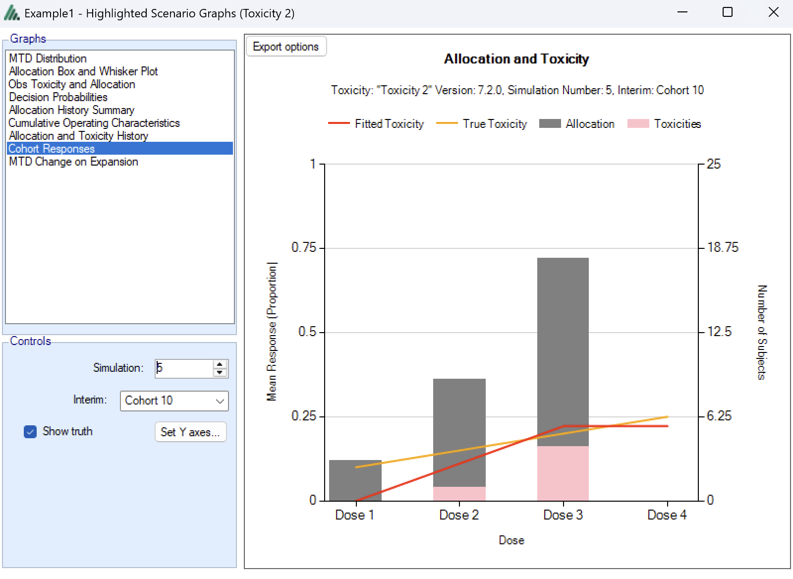
This graph shows the dose allocation and resulting toxicities along with the fitted dose-toxicity rate (based on an isotonic regression) for a single simulated trial after the results have been gathered for a specific cohort of a specific trial. Please note that isotonic regression ensures the monotonicity of the dose-toxicity relationship, but might result in the fitted toxicity rate being different (higher or lower) than the observed toxicity rate.
The graph includes a drop down selector box allowing the user to select which simulated trial is displayed, and a further drop down selector box allowing the user to select at which cohort to display the state of the trial.
These details can only be displayed for trials for which a ‘cohorts’ file has been written out.
MTD Change on Expansion
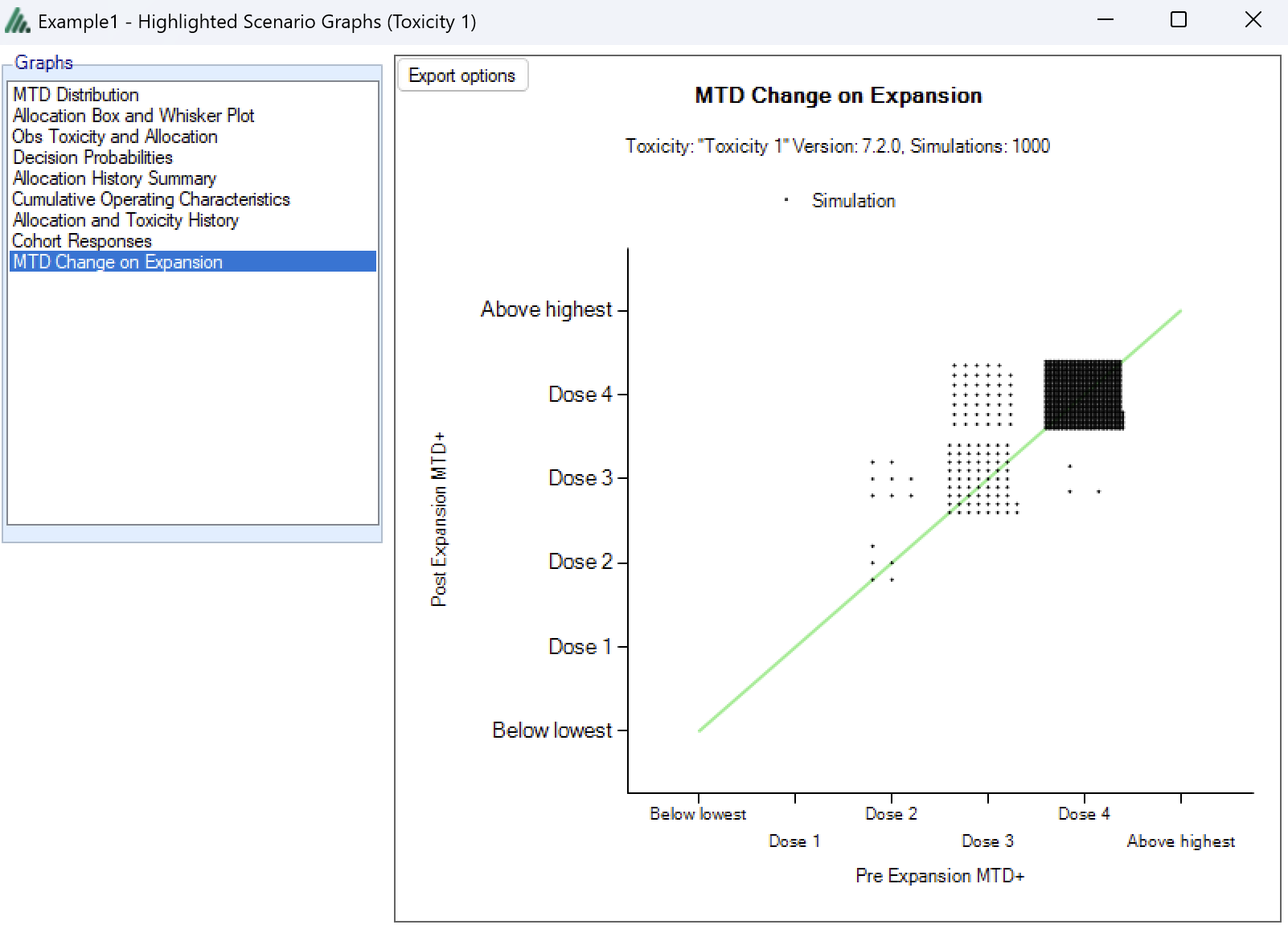
This graph plots the dose selected as MTD before the results of the expansion cohort are available, against the dose selected as MTD after the expansion cohort results are available. Each simulation result is plotted as a ‘dot’, and the graph is divided up into a grid and dots located in the correct cell in the grid and then arranged within the cell depending on how many results fall into the cell. This allows the relative number of results in each cell to be appraised quickly by eye.
This graph allows the trial designer to see the degree of risk that the determination of the MTD will change as a result of the expansion cohort and whether the risk is predominantly that the determination will increase or decrease.
There are similar graphs showing the change in the estimate of the MED and OSD after the expansion cohort.
Output Files
FACTS stores the results of simulations as csv files under a Results folder. For each row in the simulations table, there is a folder named by concatenating the names of all the different parts, which contains the corresponding csv files.
Right-clicking on a row in any of the results tables displays a context menu from which includes an option to open the results folder in explorer.
These files can be opened using Microsoft Excel, but versions before 2007 are restricted to 256 columns, which is too few to view some files in their entirety. Open Office will show all the columns and it will allow you to open two files that have the same name.
There are several types of file:
Summary.csv – contains a single row of data that holds data summarized across the simulations. This is the source of most of the values in the simulations table.
Simulations.csv – contains one row per simulation describing the final state of each simulation.
CohortsNNN.csv – contains one row for each cohort during a simulation where NNN is the number of the simulation. By default this file is written only for the first 100 simulations, but this can be changed via the advanced button on the simulation tab.