Graphs of Simulation Results
To enable swift visualization and analysis of the simulation results, FACTS has a number of pre-defined graphs it can display. Full and detailed simulation results are available in ‘csv’ format files that can be loaded into other analysis tools allowing any aspect of the simulation to be explored. These files are described below.
To view the graphs, select a row of scenario results by clicking on it and then click on the ‘View Graph’ button.
Below we have often shown full screen shots of the graphs in the graph manager, but the graph display supports copying just the graph to the clipboard to facilitate pasting them into documents and presentations. Right clicking on a graph brings up a short menu that allows the image of the graph to be copied to the clipboard or saved in ‘png’ format to a file.
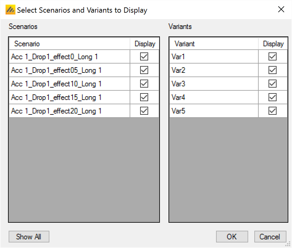
To view the graphs of the results of the simulations of a particular design variant in a particular scenario, select that row of scenario results by clicking on it and then click on the ‘View Graph’ button and select “Show Per Scenario Graphs”.
To view multiple graphs showing the results of the simulations of possibly all the design variants and all the scenarios click on the ‘View Graph’ button and select “Show Across Scenario Graphs”. This launches a graph display that displays multiple graphs in a trellis plot. You can select the graph type, filter the design variants and filter which scenarios displayed:
The graph display supports copying an image of the graph to the clipboard, to facilitate pasting them into documents and presentations. Right clicking on a graph brings up a short menu that allows the image of the graph to be copied to the clipboard or saved in ‘.png’ format to a file.
Many graphs have a number of controls to allow the graph to be tailored, standard graph controls available on most graphs are:
Set Y axis – this displays a dialog boxing allowing the user to fix the minimum and maximum of each of the Y axes and the number of ‘tick’ marks (Not displayed if the ‘y’ value must lie in the interval 0-1.)
Space doses evenly – if the x-value is ‘dose’, then data for each dose can either be spaced equally or proportionate to the doses’ effective dose strength.
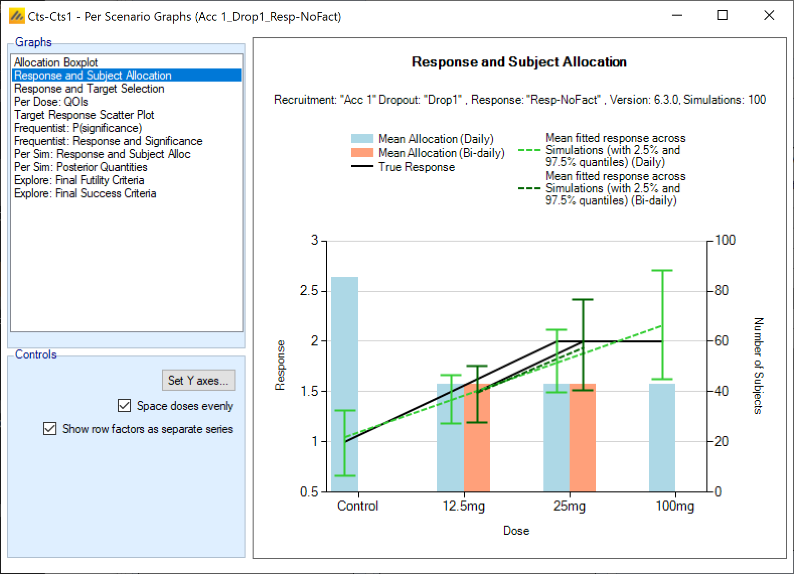
If using a 2D treatment arm model then it is possible to display graphs where the different doses (or “arms”) form the x-axis, then there is an option to show the row factors as separate series – otherwise the different combinations are displayed in effective strength order

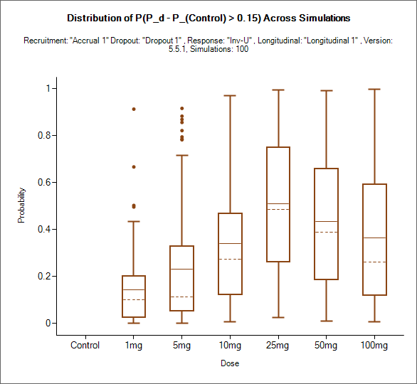
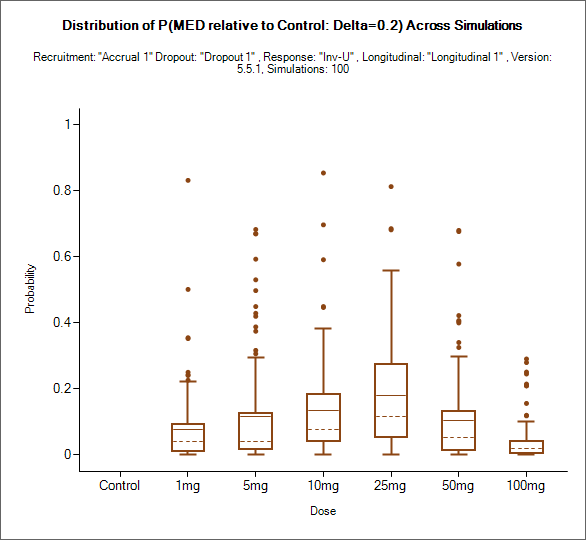
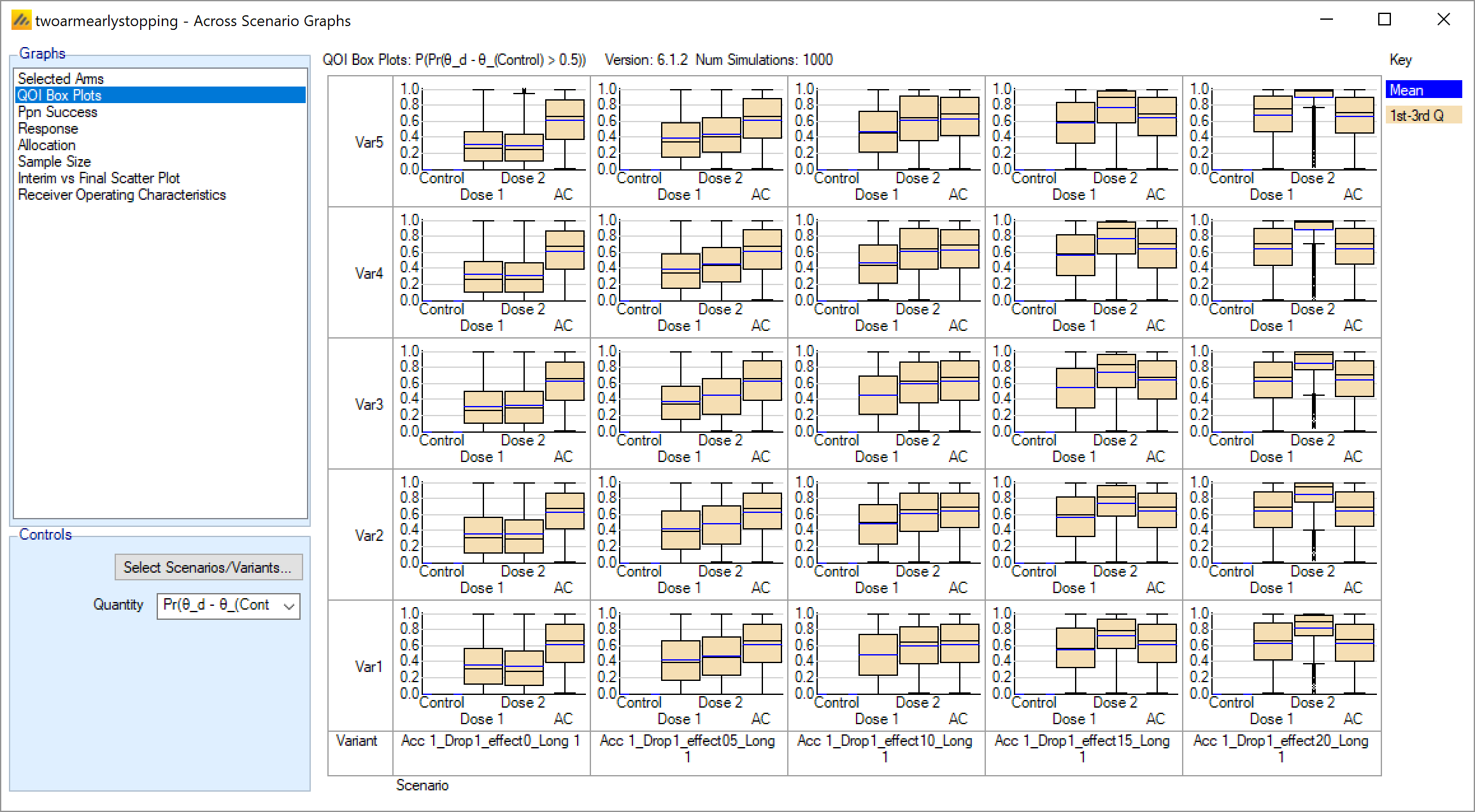
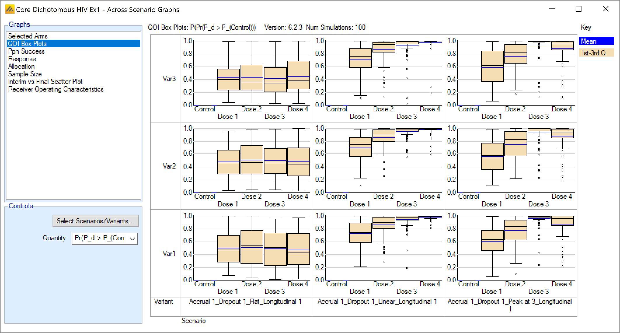
Box and whisker plot conventions
The mean probability is plotted as a large dot.
The median value is plotted as a dashed line.
The 25-75th quantile range is plotted as the “box” portion of each point.
The “whiskers” extend to the largest and smallest values within 1 ½ times the interquartile range from either end of the box.
Points outside the whisker range are considered outliers, and are plotted as small blue dots. Note that it may be difficult to see all of these symbols if they are plotted at the same value.
Per Scenario Graphs
Allocation Box and Whisker Plot
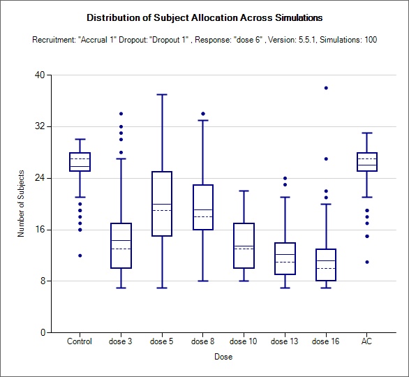
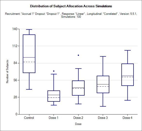
This graph displays a box and whisker plot of the number of subjects recruited into each arm. These plots show:
The distribution over all simulations of the number of subjects allocated to each arm shown as a box and whisker plot. If the design is not adaptive, the number allocated will be the same in every simulation and the box and whiskers collapse to a single line.
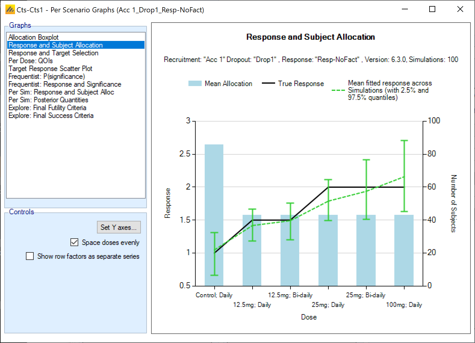
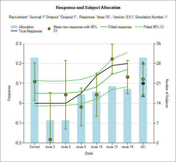
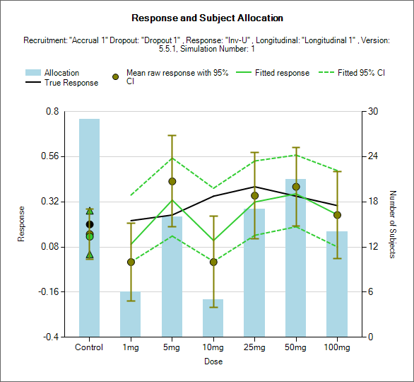
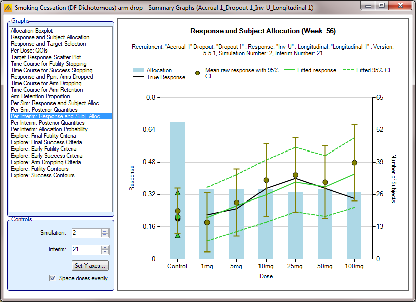
Response and Subject Allocation
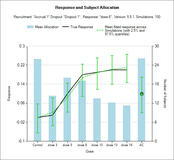
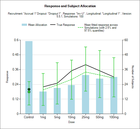
This graph shows for each treatment arm, the mean subject allocation, mean response and the 2.5%-97.5% boundaries of the estimated means over the simulations.
The blue bars show the mean number of subjects allocated.
The black line shows the true mean response being simulated.
The green dashed line shows the mean of the estimated response across the simulations
The green ‘error bars’ show the spread of the central 95% of the estimated mean response across the simulations (if less than 20 simulations have been run it simply shows the full spread).
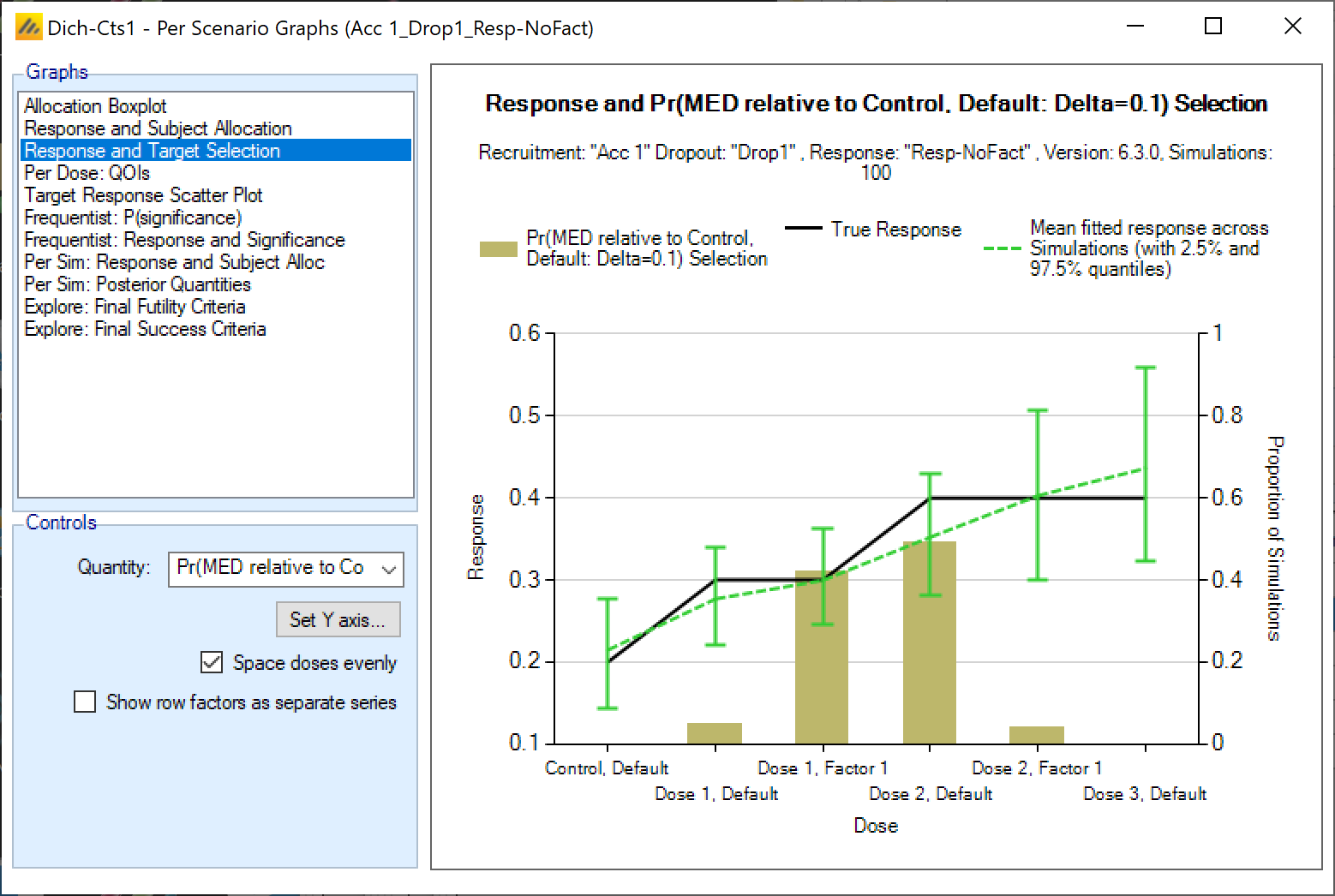
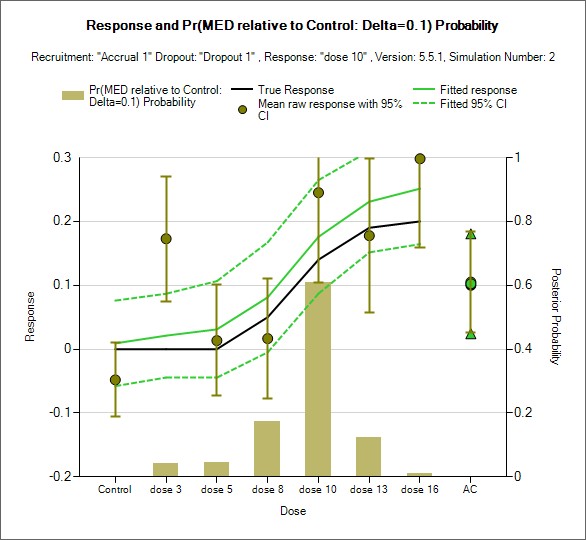
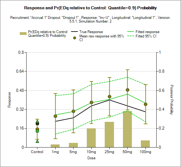
Response and Target Selection graphs
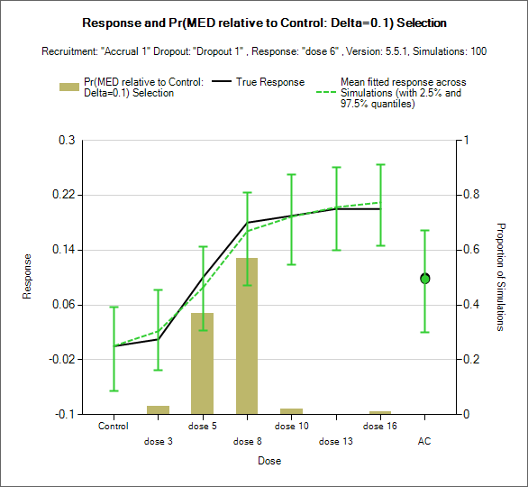
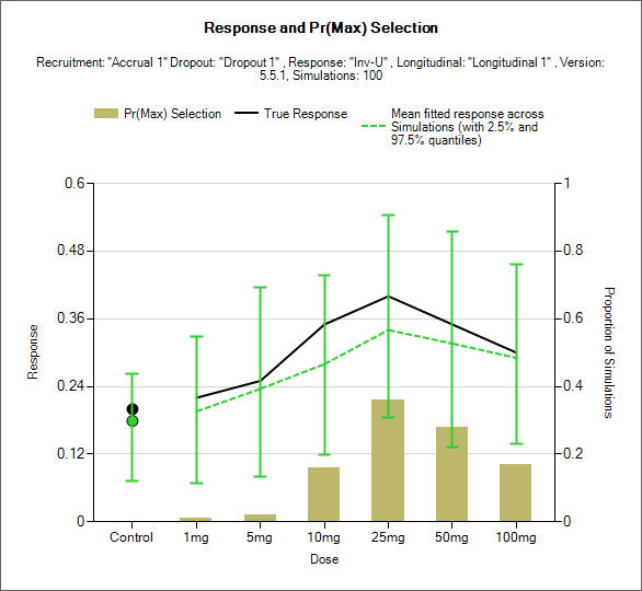
These plots show the true simulated mean response and the mean and 95% spread of the mean fitted mean responses along with bars showing the proportion of simulations the different treatment arms are the selected target arm for each of the “Probability of being target” QOIs, such as Pr(Max), Pr(EDq relative to ..: Quantile=q) and Pr(MED relative to…: Delta=\(\delta\)).
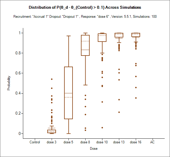
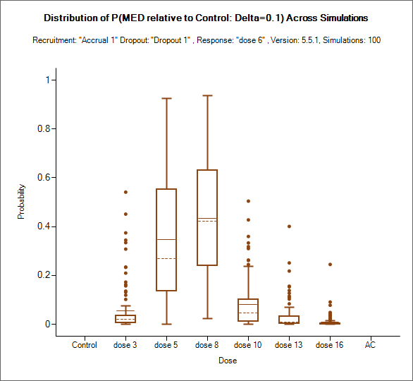
Per Dose QOIs (Box and Whisker Plots)
This set of graphs show the distribution over the simulations of the posterior probability estimates of quantities of interest for each dose. All the Posterior Probability, Predictive Probability, P-value and Probability of being Target QOIs that have been defined are available for plotting, via a drop down list.
Note that in any one analysis the Probability of being Target will sum to 1 across the doses (and can sum to less than one in the case of the MED target if none of the doses look likely to be better than the CSD), whereas all the other QOIs are assessed individually for each dose.
Target Response by Sample Size Scatter Plot
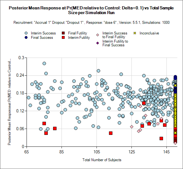
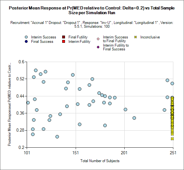
This graph shows a scatter plot of trial outcomes with the selected Target QOI as the y-axis and total number of subjects recruited as the x-axis. The trials are plotted with a symbol that indicated the final outcome:
A light blue circle indicates a trial that stopped early for success
A dark blue circle indicates a trial that was a late success
A dark red square indicates a trial that was a late futility
A light red square indicates a trial that stopped early for futility
A light pink diamond indicates a trial that stopped early for success but where the final analysis was futility
A dark pink diamond indicates a trial that stopped early for futility but where the final analysis was success
A yellow cross indicates a trial that completed full enrolment but was inconclusive at the end.
These graphs are not particularly useful if there is no early stopping.
If the design does allow early stopping this graph shows
The overall distribution of sample sizes – in particular is stopping evenly distributed from the moment stopping is possible, or is there are large cohort of trials that stop as soon as it is possible?
When and with what mean response trials stop incorrectly, in particular having trials stopping and the decision being reversed suggests stopping is allowed to soon or the criteria is not conservative enough.
Cumulative Operating Characteristics Plot
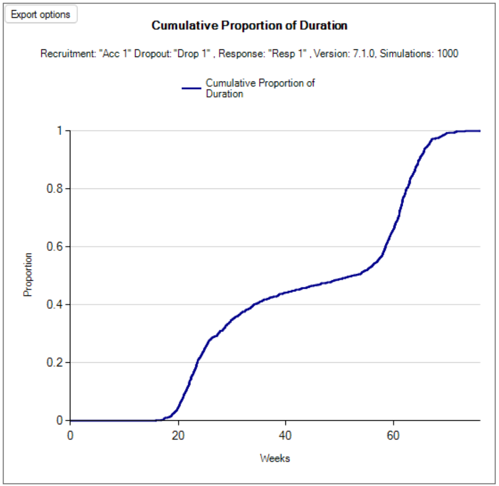
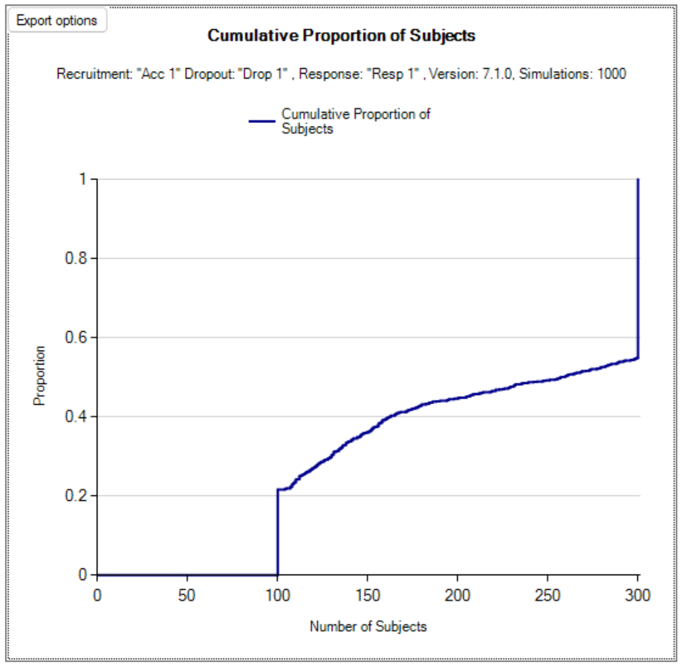


There are two graphs, one that shows the cumulative proportion of durations across all simulations, and the other shows the cumulative proportion of subjects across all simulations.
Time course for stopping
There are two graphs, one that shows the distribution over time for stopping for futility and one for stopping for success.
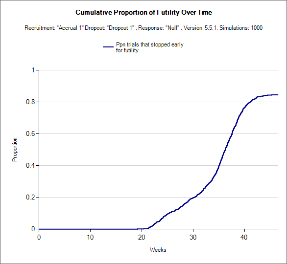
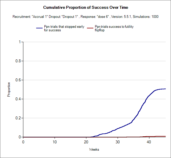
These plots show as cumulative curves the proportion of the simulations that stopped at different time points from the start of the trial. The user can select whether time or subject enrollment is used as the x-axis.
Arm Dropping Graphs
If the design has used arm dropping, the following graphs are available.
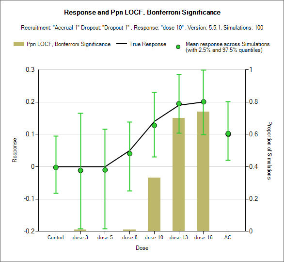
Response and Ppn Arms Dropped
This graph shows the true (simulated) mean response and the average fitted response with 2.5% & 97.5% quantiles.
The histogram bars show for each arm the proportion of simulations for which the arm was dropped.
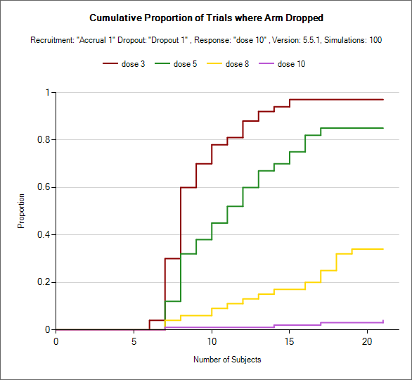
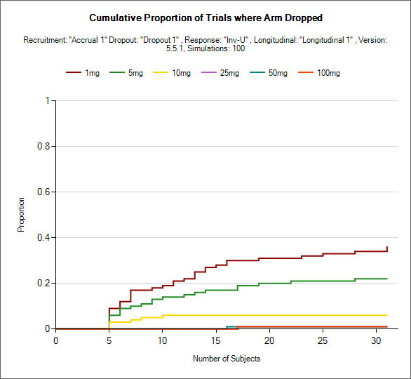
Time Course for Arm Dropping
This graph shows, for each arm, the cumulative proportion of simulations when it was dropped. The user can select whether time or number of subjects allocated to the arm is used as the x-axis.
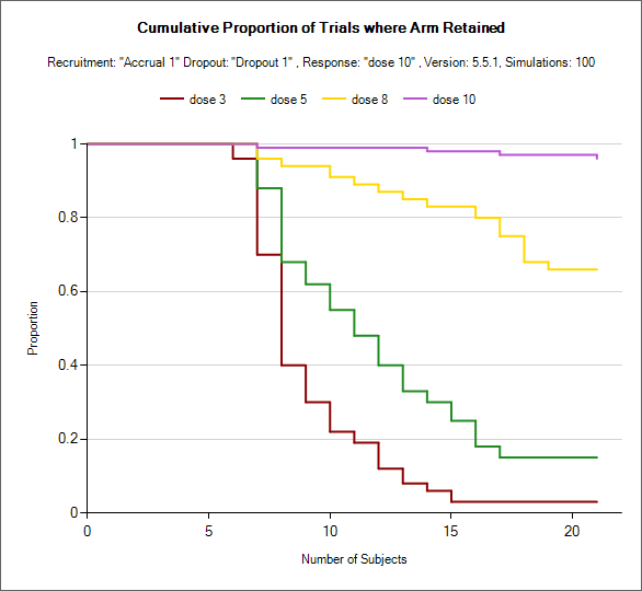
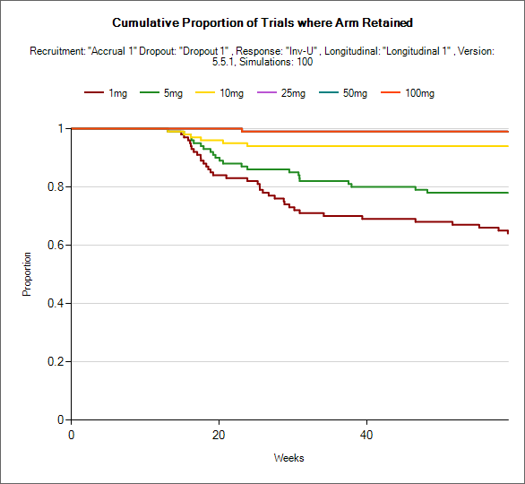
Time Course for Arm retention
This graph shows, for each arm, the cumulative proportion of simulations when the arm was retained. The user can select whether time or number of subjects allocated to the arm is used as the x-axis. This is simply the inverse of the arm dropping graph above.
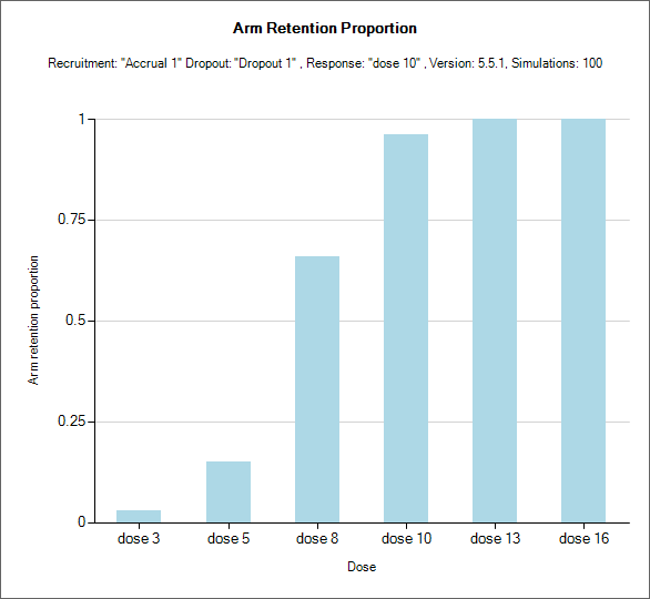
Arm Retention Proportion
This graph shows, for each arm, the simple proportion of simulations where the arm was retained.
Frequentist
These graphs are available if frequentist analysis is enabled.
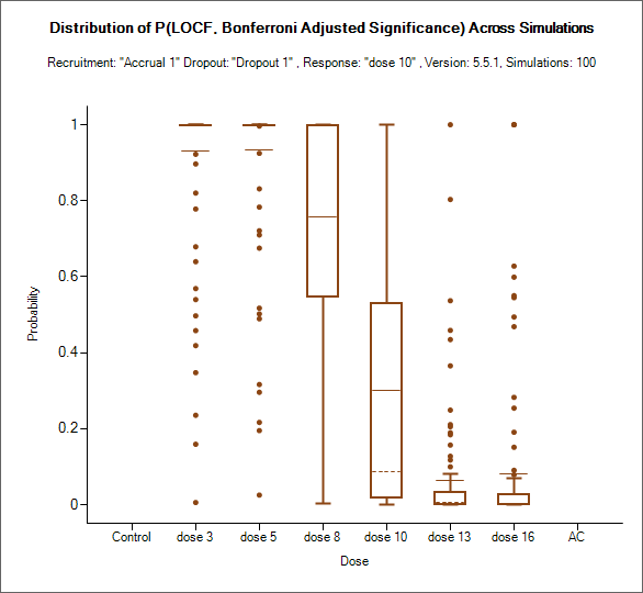
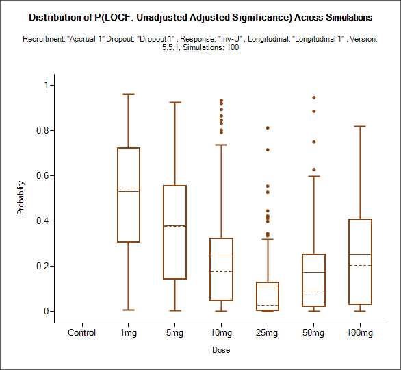
Frequentist P(significance)
These graphs are the box and whisker plots of various p-values that are automatically calculated (that is to say they do not need to be defined as QOIs for them to be calculated) for the final analysis. The user can select from Unadjusted, Bonferroni and Dunnett's and LOCF, BOCF (if baseline is simulated) or PP (per-protocol) treatment of missing values.
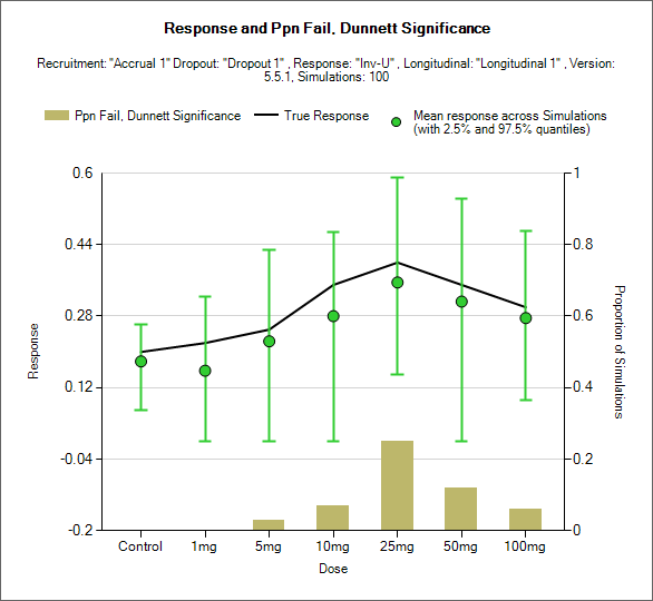
Frequentist: Response and Significance
This graph plots the mean and 2.5-97.5 percentile of the mean across the simulations or the simple frequentist estimate of the response for each arm, along with a histogram plot of the ppn of times the response on each arm was significant. The user can select from Unadjusted, Bonferroni or Dunnett’s and LOCF, BOCF (if baseline is simulated) or PP (per-protocol) treatment of missing values.
Per Sim: Response and Subject Alloc
This graph shows the final analysis at the end of individual simulations.
This graph includes a control that allows the user to select which simulation to graph the results from. On each graph
The black line shows the ‘True’ mean response being simulated.
The brown circles and arms show the mean raw data and its 95% CI for each arm.
The green solid line shows the estimate of the mean response.
The green dashed lines show the boundaries of the 95% credible interval for the estimate of the response.
Blue bars showing the number of subjects allocated on each treatment arm.

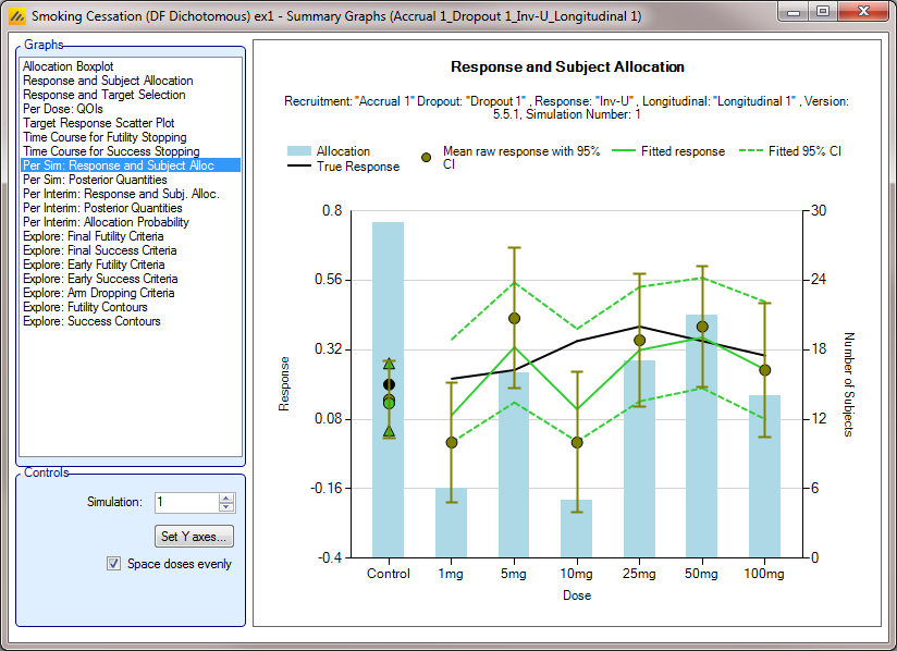
Control to select the individual simulation results to be displayed
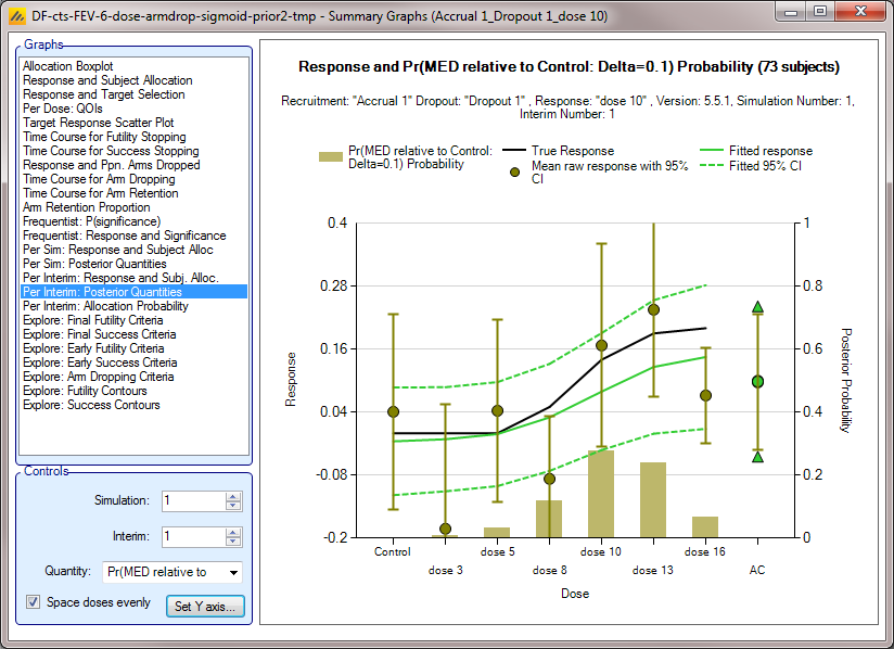
Per Sim: Posterior Quantities
This graph shows the final analysis at the end of individual simulations, including the distribution of a selected QOI.
This graph includes a control that allows the user to select which simulation to graph the results from. On each graph
The black line shows the ‘True’ mean response being simulated.
The brown circles and arms show the mean raw data and its 95% CI for each arm.
The green solid line shows the estimate of the mean response.
The green dashed lines show the boundaries of the 95% credible interval for the estimate of the response.
Brown bars showing the final value of the selected QOI for each arm at the end of the simulated trial.
The user can select from any of the Posterior Probability, Predictive Probability or Target Probability QOIs to plot.
Per Interim Response Graphs
This is an identical set of graphs to the Per Sim graphs, the difference is that in addition to a control to select which simulation to graph the results from, there is a control to select which interim within the simulation to graph the results from. These graphs are only available for those simulations for which ‘weeks’ files have been output (by default the first 100).
Note the ‘Interim’ control in both of the below figures.
Post Simulation Boundary Finding Graphs
Explore Success/Futility Criteria
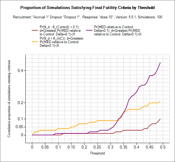
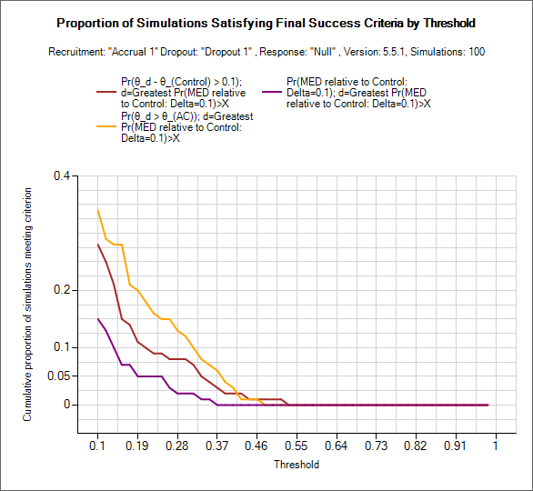
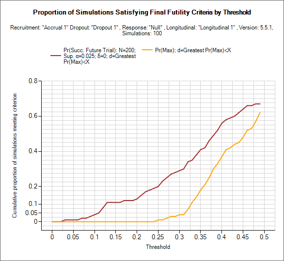
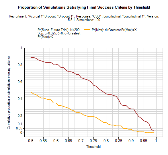
These graphs can be used to explore what proportion of simulated trials of a particular scenario would have been a success/failure at final evaluation. Using the two drop down controls the user can select the target dose to use: e.g. Pr(Max), and set and lower/upper limits to explore for the threshold (setting the range used on the x-axis). The graphs show for all the decision QOIs defined for the selected Target Dose the proportion of simulations that would have met the threshold values.
As in the examples above, the plots will be somewhat jagged if only a small number of simulations have been run. These graphs can be used to select thresholds that can be expected to yield a certain level of type-1 or power, but the user must remember these will only be approximate (depending on the number of simulations) but can be useful to understand the designs sensitivity to the thresholds and to set initial thresholds early on in the design / simulation process that will get close to the desired type-1 error and power from the outset.
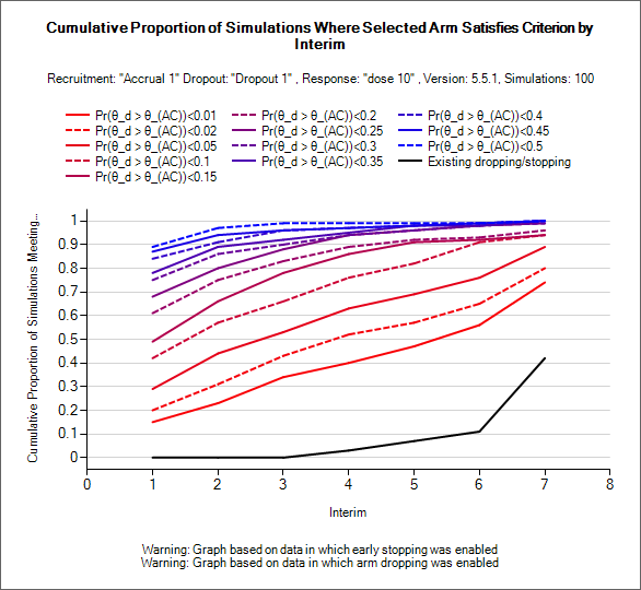
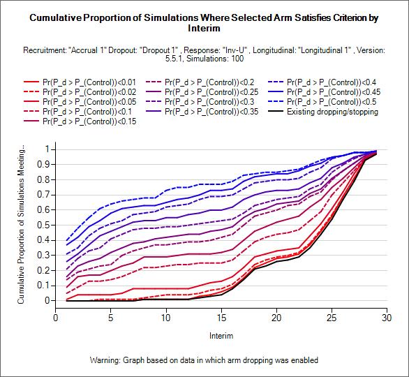
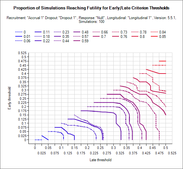
Explore Early Success/Futility Criteria
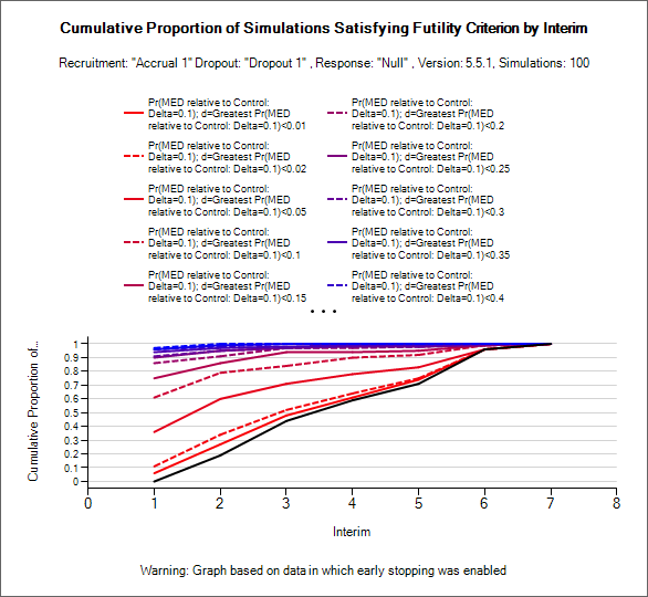
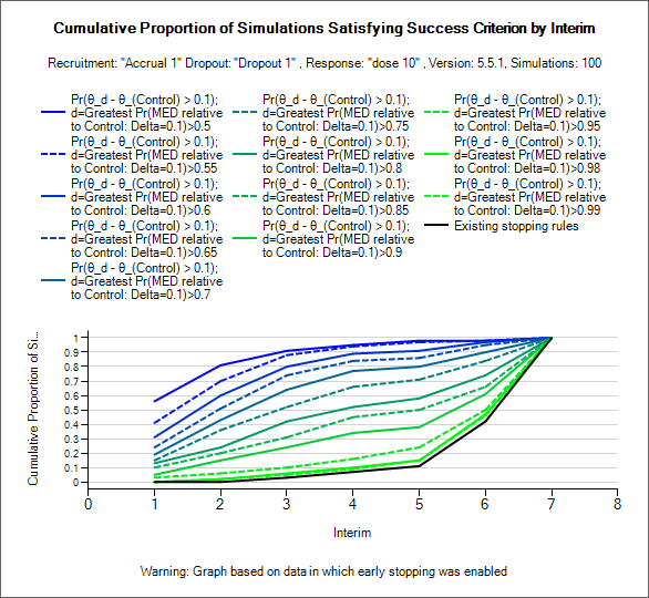
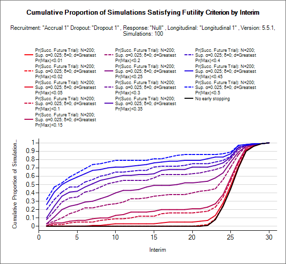
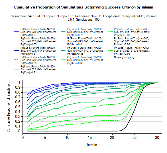
These graphs can be used to explore what proportion of simulated trials of a particular scenario would have stopped early for success/futility. NOTE these graphs require weeks files to have been output, they are also most use where the design has been simulated with interims but no early stopping (unlike the examples above where the shape of the “existing stopping rules” line indicates that early stopping occurred in these simulations).
Using the two drop down controls, the user can select which decision QOI is evaluated and from which interim onwards stopping will be permitted. Lines are then displayed for the proportion of simulations that would have stopped by each interim for a fixed set of thresholds.
Typically these can be used to see at what threshold (and starting at what interim) stopping for success or futility introduces an unacceptably level of ‘incorrect’ early stopping – stopping for futility in successful scenarios and stopping for success in futile scenarios and whether at below/above these levels there may be a useful probability of correct stopping.
Explore Arm Dropping Criteria
This graph is similar to the Explore Early Success/Futility Criteria graph but for arm dropping criteria. The user has an additional control to select which dose the proportion of trials in which the arm would be dropped is displayed.
Success/Futility Stopping Contours
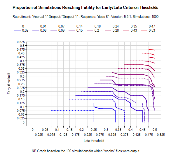
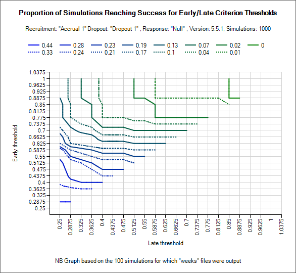
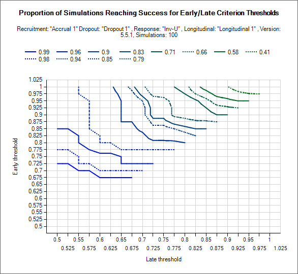
These graphs allow early stopping and final evaluation criteria to be considered jointly. Like the explore early stopping criteria plots, these graphs require weeks files to have been output and will work best if interims were evaluated but no trials actually stopped early.
The user selects the decision QOI to plot, the first interim at which early stopping is allowed, and the upper/lower limit of the threshold to consider.
FACTS will then plot contours where (final evaluation threshold, early stopping threshold) yield the same proportion of trials that are successful/futile. Contours are only plotted where final evaluation threshold < early stopping threshold for success and vice versa for futility. Early stopping criteria should not be less strict than final criteria.
Again the example graphs shown are based on only 100 simulations with weeks files, so any threshold derived will only very approximately yield these success/futility rates.
MCMC Trace plots
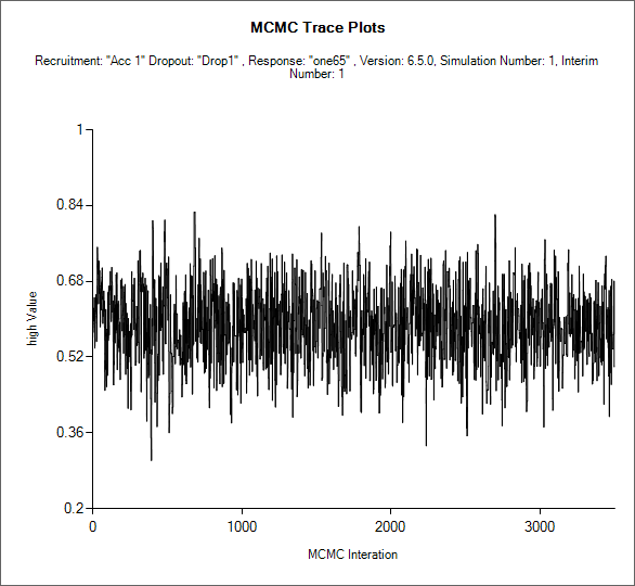
If an MCMC sample file has been output for one or more simulations (the default is to not output MCMC sample files due to their size), then for each of those simulations it is possible to view the MCMC trace of the sampled values for each of the parameters sampled in the MCMC.
If the design is adaptive, the user can select which interim (“update”) the samples are from, as well as which parameter’s samples to plot.
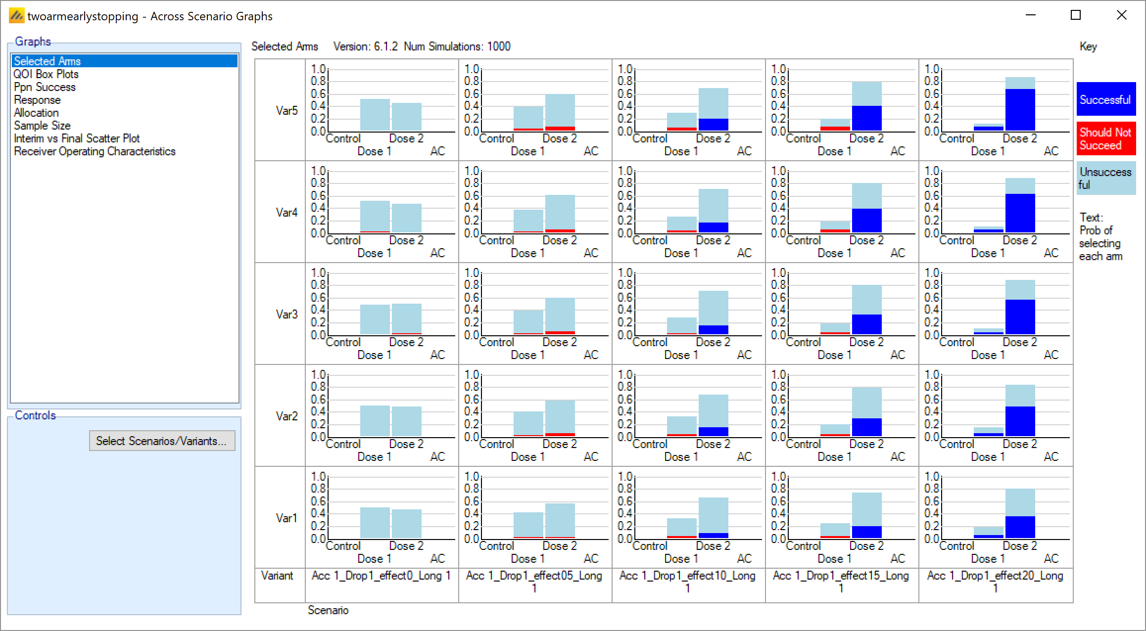
Across Scenario Graphs
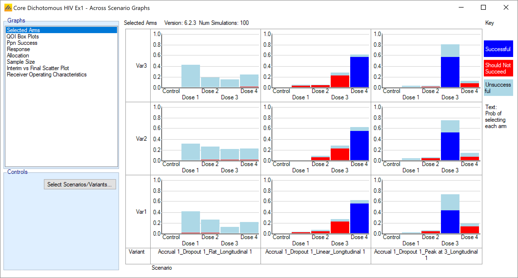
Selected Arms
This graph shows a bar chart for each scenario and variant selected. Each chart shows how often each arm was ‘selected’ by the target QOI specified on the Study > Variants tab. Each bar uses a stacked bar to show the proportion of times that arm was:
“Successful” –the arm was correctly selected (marked as “Should succeed” on the VSR tab) and the trial was successful.
“Should not succeed” – the arm was incorrectly selected (not marked as “Should succeed” on the VSR tab) and the trial was successful.
Unsuccessful – the arm was selected and the trial failed.
QOI Box Plots
This graph shows a box and whisker plot for each scenario and variant selected. Each plot shows the distribution of the values of a selected QOI for each arm. There is a drop down control to allow the selection of the QOI to be displayed. Any Posterior probability, Predictive probability, p-value or target QOI can be selected.
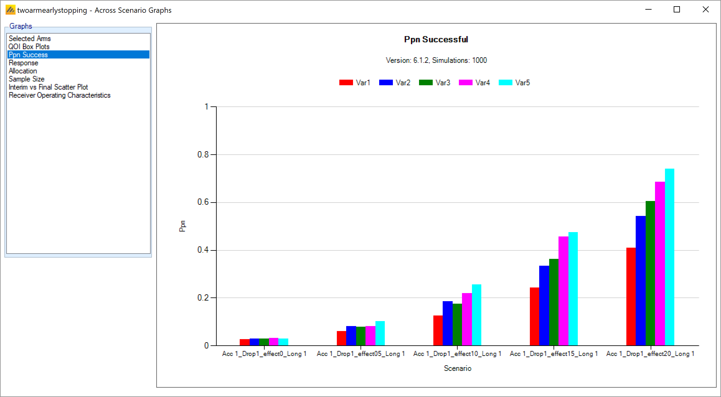
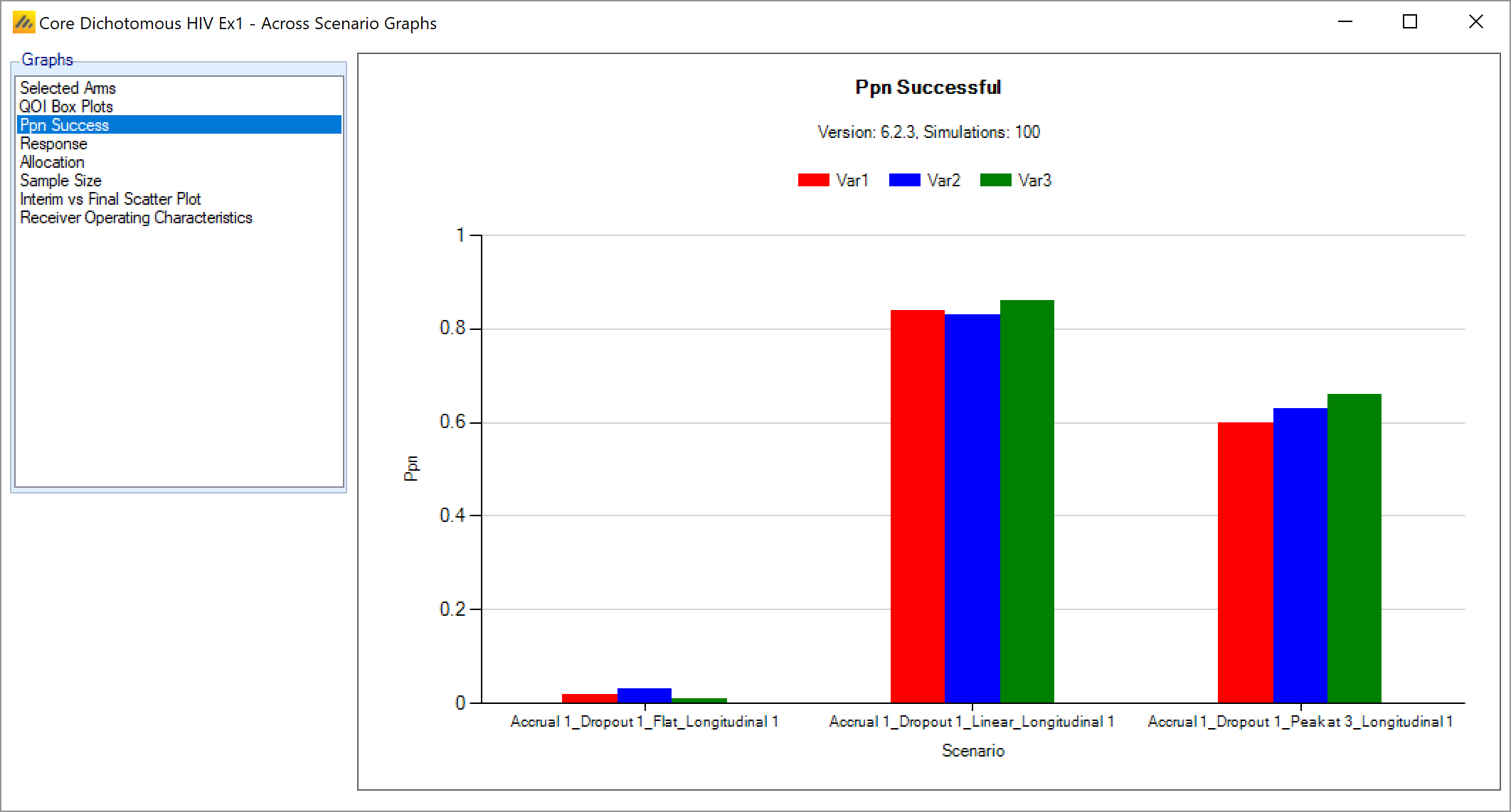
Ppn Success
This grouped bar chart shows a bar for the proportion of successful simulations for each variant, grouped by scenario.
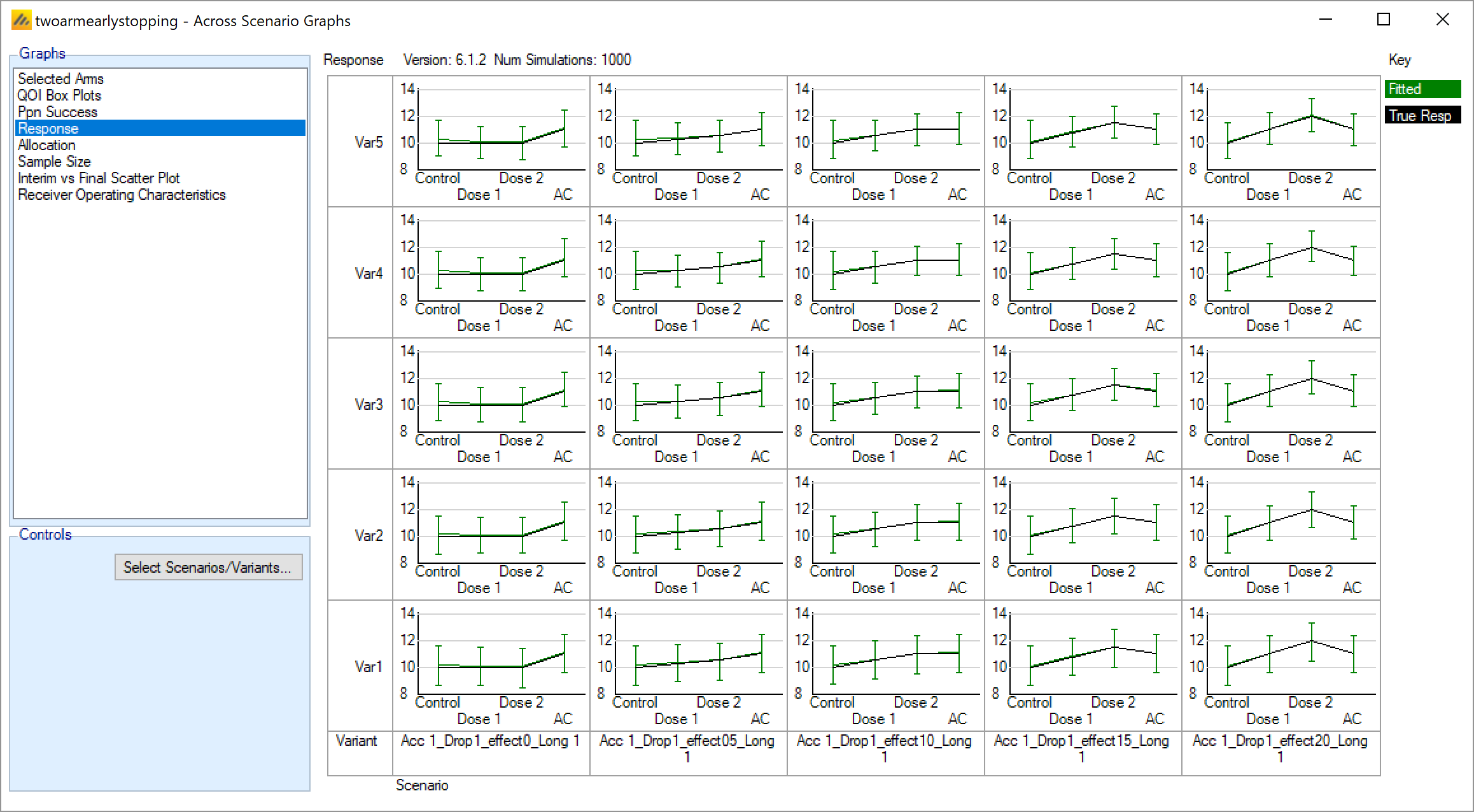
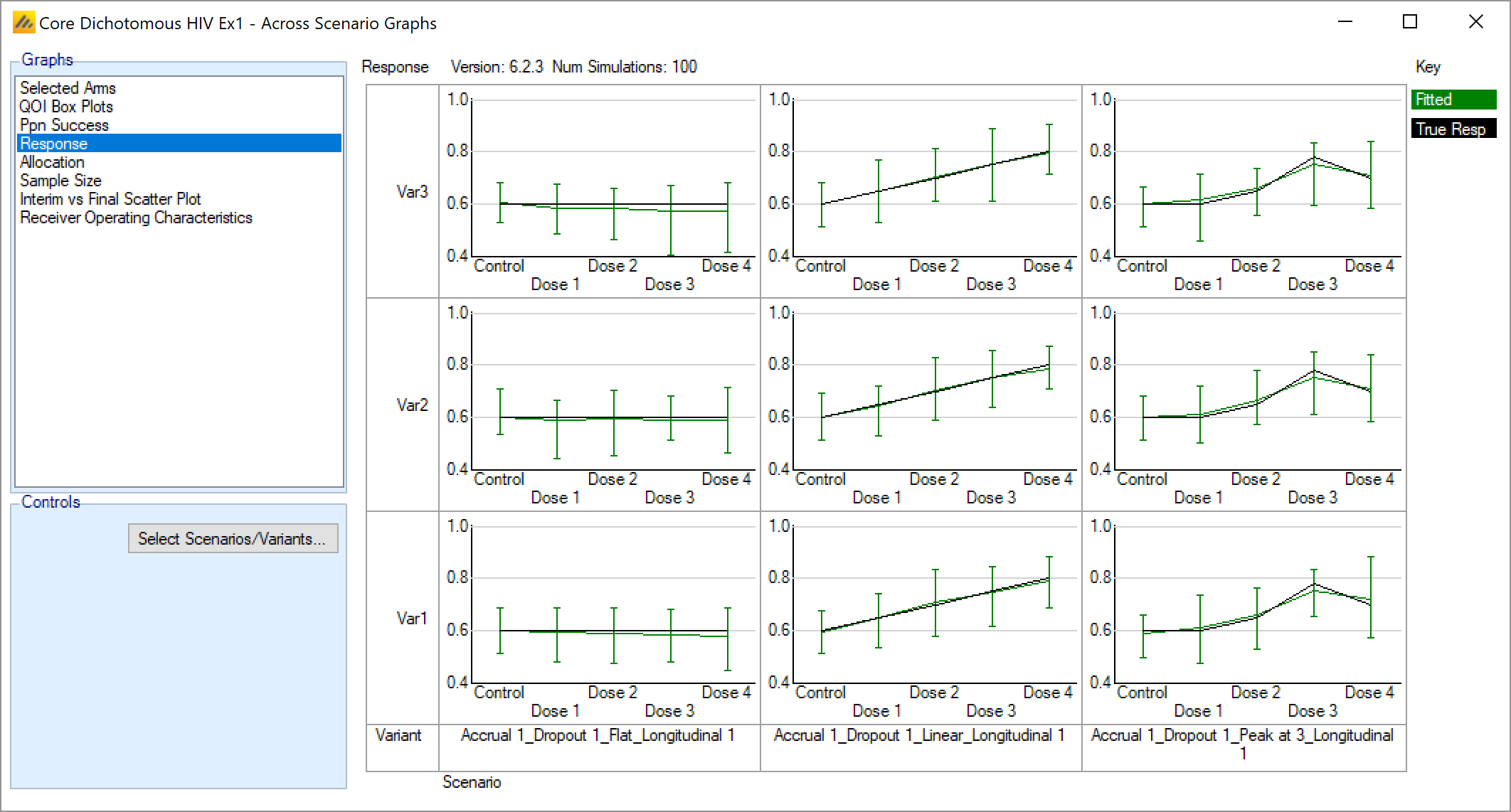
Response
This graph shows a dose response plot for each scenario and variant selected. Each plot shows the mean estimate over the simulations and the 95%-ile interval of the mean estimates over the simulations. The graph also shoes the “true response” i.e. the mean response being simulated.
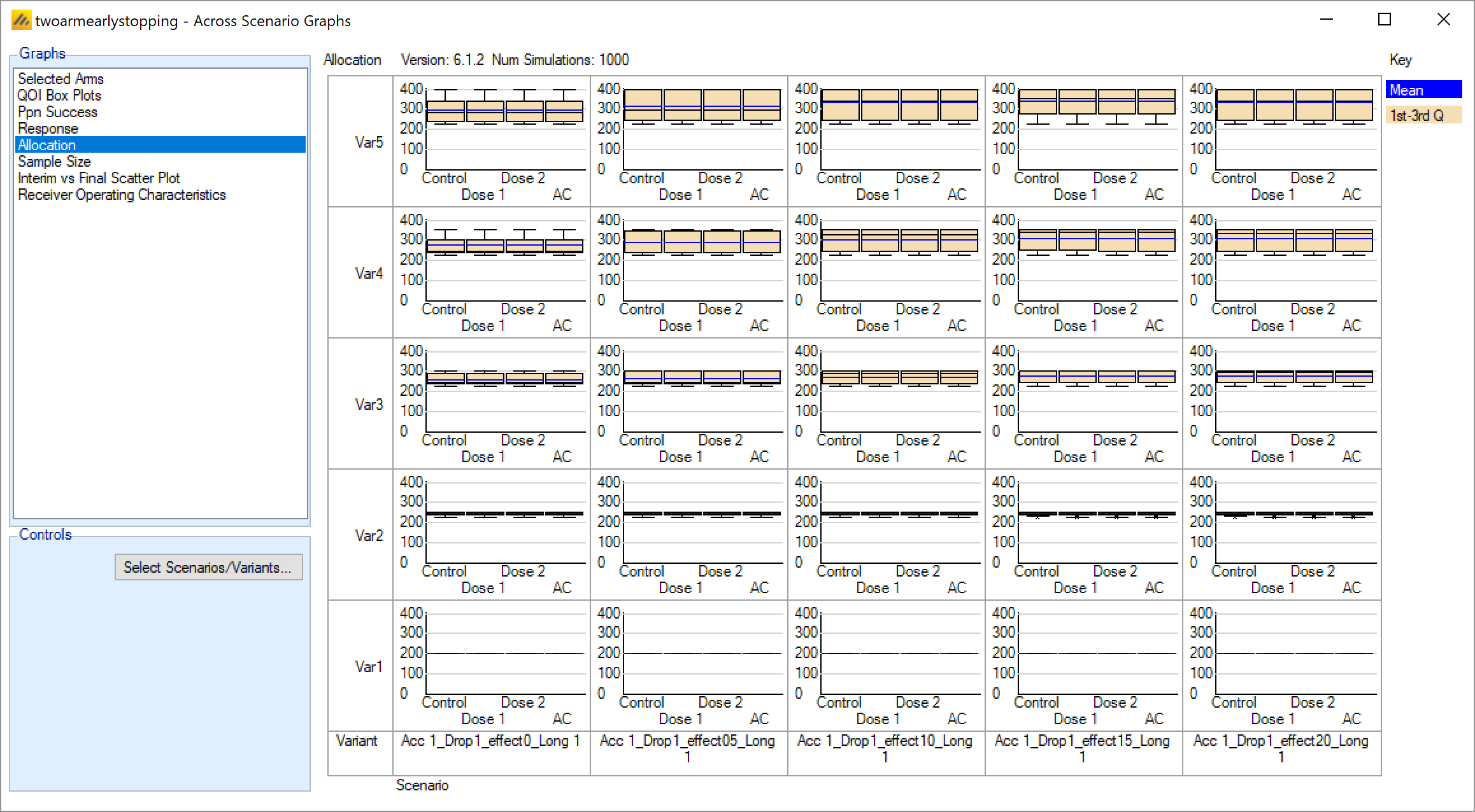
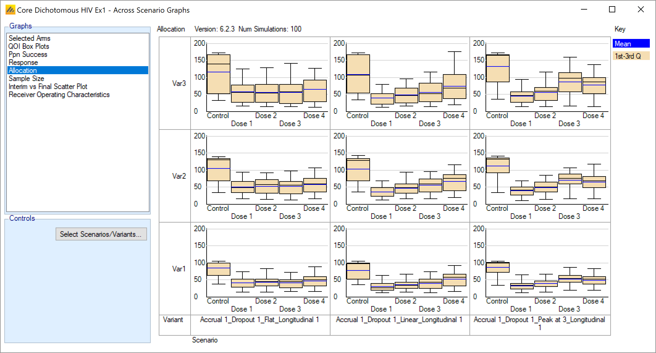
Allocation
This graph shows a box and whisker plot for each scenario and variant selected. Each plot shows the distribution of the number of subjects allocated to each arm over the simulations.
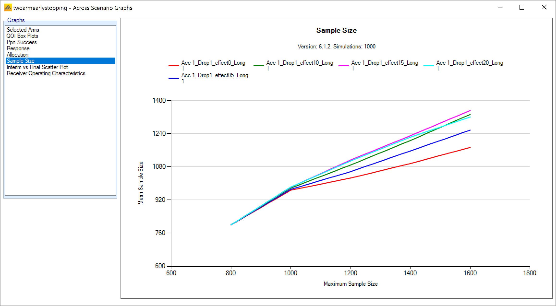
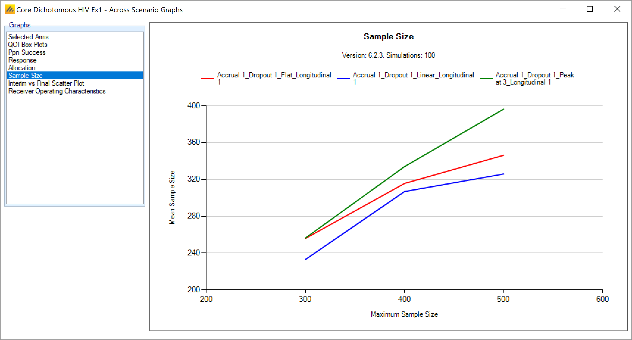
Sample Size
This graph shows the mean sample size for each scenario at different maximum sample sizes (the different variants).
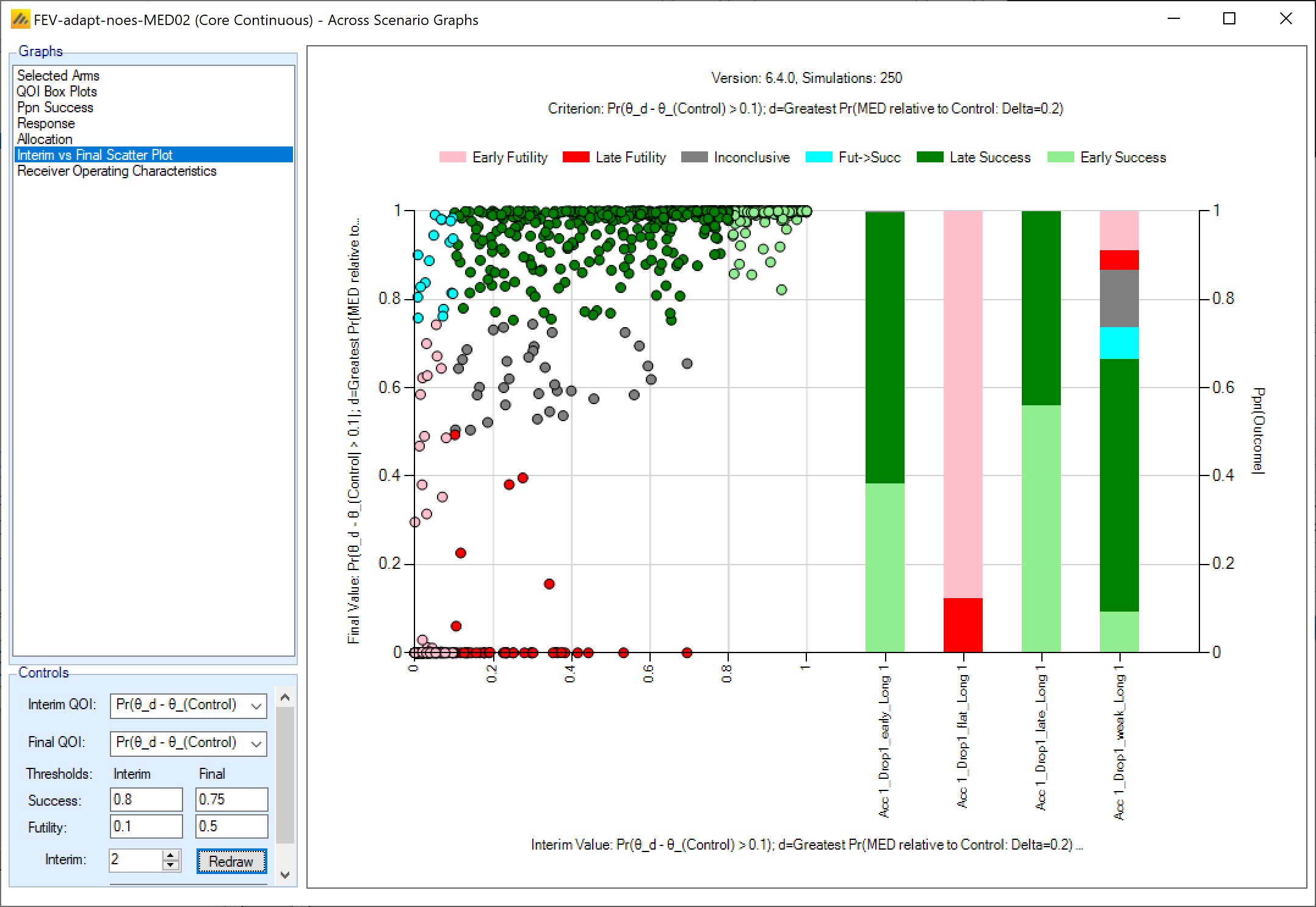
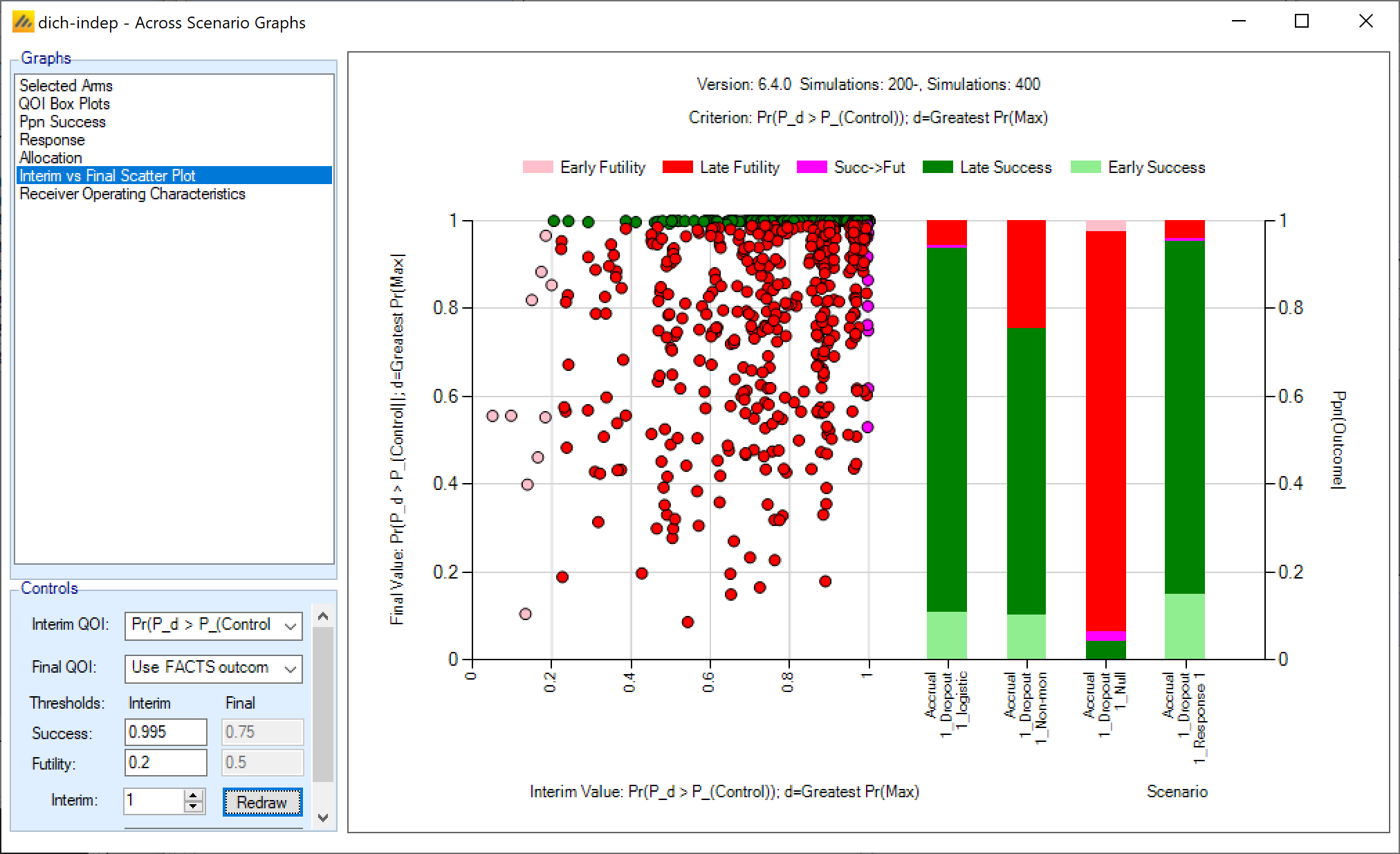
Interim vs Final Scatter Plot
This is an interactive plot that shows the outcome of each simulation over all the scenarios of a selected variant.
The x-axis shows the value of the selected decision QOI at the specified interim, and the y-axis shows the final value of a (possibly different) selected decision QOI. As well as selecting a decision QOI for the final decision, the graph can use the actual final decision in the simulations – the value of the QOI used in the first criteria is used for the decision is used for the y-axis.
Note the graph is based just on the values at the selected interim, what might happen at other interims is ignored.
Thresholds can be set to specify early and late success/futility. Each scenario is then coloured to show its outcome – and stacked bar graphs are displayed to show the proportion of each outcome for each scenario. The thresholds can be changed and the graph re-drawn. If the selected QOI uses a p-value the checks for success are that it is “<” than the threshold, (and vice-versa for futility), otherwise the checks for success are that it is “>” the threshold (and vice-versa for futility).
The graph can only display the results for simulations for which cohorts files have been output, and for simulations that reached the specified interim. Thus the graph works best if interims have been specified, but the simulations run without any early stopping enabled – so each simulation has the results for every interim.
With 1,000 simulations per scenario and cohorts files for each simulation, the graph will take several seconds to re-draw. To allow several parameters to be set before redrawing (rather than having to wait for the redraw after each change) the graph is only redrawn after the ‘Redraw’ button is clicked.
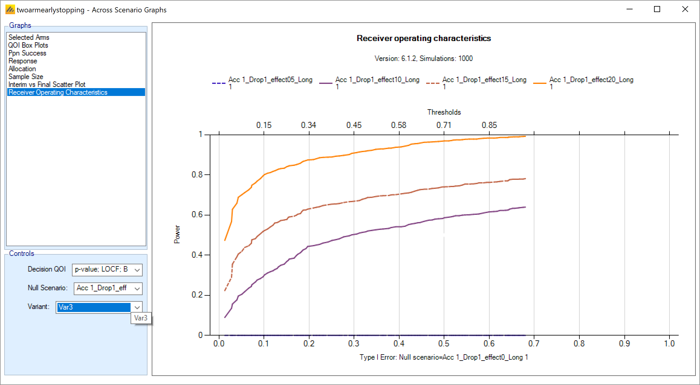
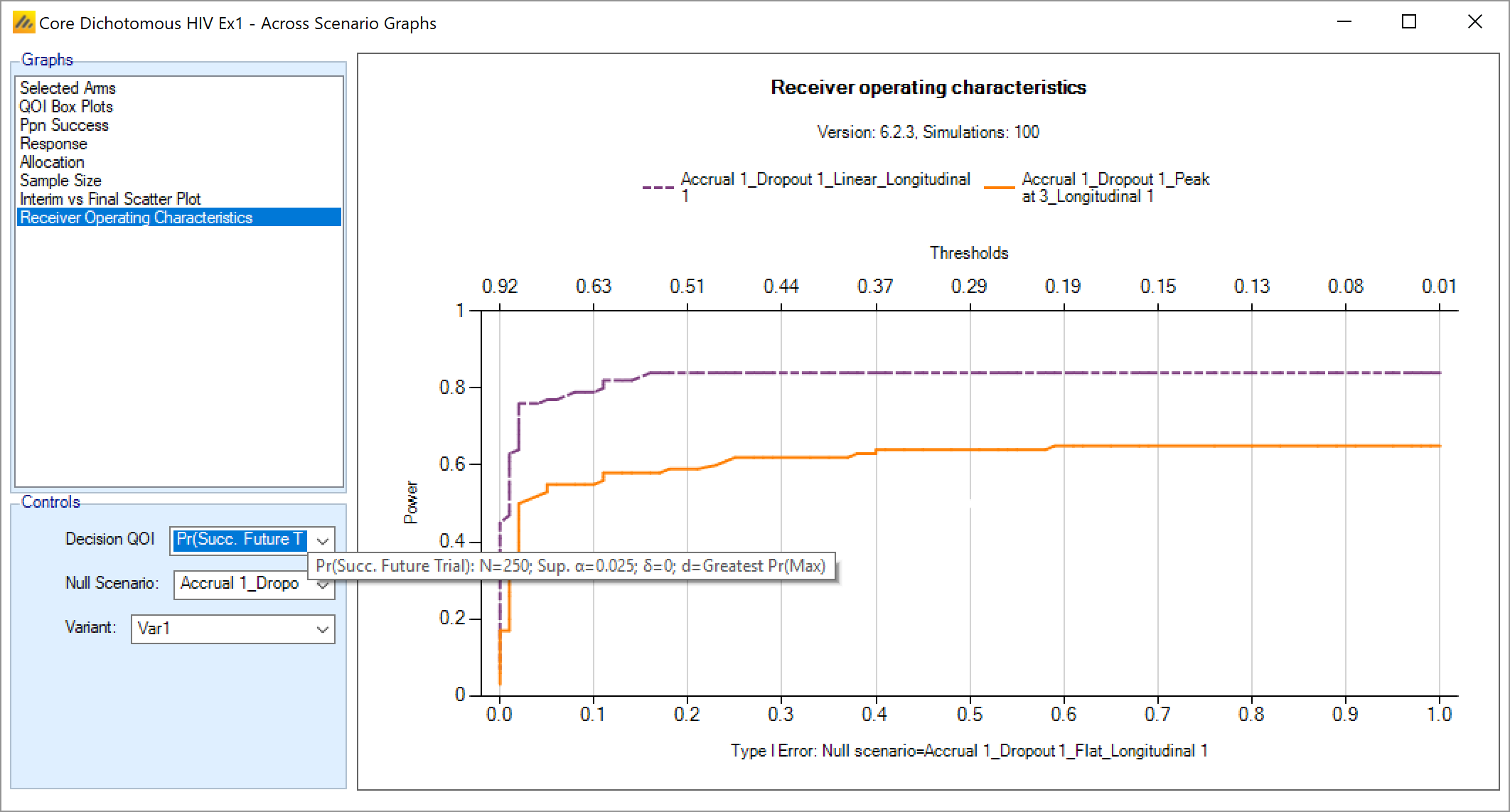
Receiver Operating Characteristics
This graph plots the relative proportion of successful simulations in the scenarios compared to the proportion of successes in one specific scenario. The intended use of this is to yield a “Receiver Operating Characteristics” (ROC) curve. This is done as follows:
Select the decision QoI that is to be used to determine final success/futility. (The graph only supports the simple case where just one is being used).
Select a scenario that represents the ‘Null’ case – where determining success is a type-1 error.
If multiple variants have been simulated, select which variant to plot.
FACTS computes for the null scenario, for a range of decision threshold values, what proportion of the ‘Null’ scenario sims would have been successful (giving the estimated type-1 error rate), these proportions form the x-values for each point. The corresponding threshold values are shown on the x-axis at the top of the graph, the type-1 error rate on the x-axis at the bottom of the graph.
FACTS then computes for each of the other scenarios in turn the proportion of sims that would have been successful and selected a “should succeed” dose so it is necessary for doses to have been specified as “should succeed” on the Virtual Subject Response profiles (giving the estimate of power for that scenario – where ‘power’ also requires correct dose selection), at each of the threshold values, these proportions are then shown on the y-axis of the graph.
Thus for each scenario we can see the estimated power of the design to determine success for a given type-1 error rate in the specified Null scenario.
Viewing Simulation Results in the Simulations Tab
After simulations have been run, FACTS provides a table for assessing the output from the simulations. While everything that FACTS displays in the table on the Simulation tab is available in output files, FACTS does a substantial amount of “beautifying” of results in its built-in table. This entails changes like converting numeric outcome scores to readable text and using descriptive names for QOI columns.
The main table has 1 line per scenario, and shows the summary of all simulations run for each scenario. These lines show values that are stored in the summary.csv file.
More detailed simulation output, providing a row per simulation run, is accessibile by double clicking on any row of the output table. This row-per-simulation output is what is stored in the simulations.csv files.
Additional detail is available for simulations that have a weeks file by right clicking on a simulation in the simulation summary window and selecting “Weeks Results”. See the Results Output section of the Simulation tab to specify the number of weeks files to be output.
Summary per Scenario
By default, only a subset of all columns of output are provided when simulations are complete. This set of columns is called “Highlights.” To get access to further columns, you can right click anywhere on the simulation output table and click “Summary Results: ….” for whichever set of columns you would like to see. There is a “Summary Results: All” option that will provide a pop up containing every column available for summary results.
The following sections break down which columns are available by sorting to which column subset.
Highlights
These are the columns displayed on the simulations tab after simulations are completed, the can also be displayed in the separate “Highlights” results window.
| Column Title | Number of columns | Description |
|---|---|---|
| Select | 1 | Not an output column, this column contains check box to allow the user to select which scenario to simulate. The ‘Select All’ button causes them all to be checked. |
| Status | 1 | This column reports on the current status of simulations: Completed, Running, No Results, Out of date, Error. It is updated automatically. |
| Scenario | 1 | This column gives the name of the scenario, concatenating together the profile names from the following tabs: ‘Execution > Accrual’, ‘Execution > Dropout Rate’, ‘Virtual Subject Response > Explicitly Defined > Dose Response’, ’Virtual Subject Response > Explicitly Defined > Control Hazard rates, ‘Virtual Subject Response > Explicitly Defined > Predictor’, This is the same name as used for the results directory |
| Random Number Seed | 1 | Base random number seed used to perform the simulations. |
| Num Sims | 1 | The number of simulations that were run to produce the displayed results. |
| Mean Subj. | 1 | This is the mean (over the simulations) of the number of subjects recruited in this scenario. |
| Ppn Overall Success | 1 | This is the proportion of simulations that stopped for success, either early success or late success (as defined below). |
| Ppn Early Success | 1 | This is the proportion of simulations that stopped early for success (and did not regress to futility in the final analysis – though they might have regressed to ‘inconclusive’). |
| Ppn Late Success | 1 | This is the proportion of simulations that did not stop early but were successful in the final analysis. |
| Ppn Overall Futility | 1 | This is the proportion of simulations that stopped for futility, either early futility or late futility (as defined below). |
| Ppn Late Futility | 1 | This is the proportion of simulations that did not stop early but were futile in the final analysis. |
| Ppn Early Futility | 1 | This is the proportion of simulations that stopped early for futility (and did not regress to success in the final analysis – though they might have regressed to ‘inconclusive’). |
| Ppn S uc->Fut Flipflop | 1 | This is the proportion of simulations that stopped early for success but regressed to futility in the final analysis. |
| Ppn F ut->Suc Flipflop | 1 | This is the proportion of simulations that stopped early for futility but regressed to success in the final analysis. |
| Ppn Inco nclusive | 1 | This is the proportion of simulations that did not stop early and were neither successful nor futile in the final analysis. |
| Early Success Time | 1 | This is the average time to an early decision to stop for success (i.e. the time excluding final follow up) over those simulations that did decide early to stop for success. |
| Mean Trt. <Dose> | One per arm | This is the mean (over the simulations) of the hazard ratio of the treatment arms to control. The HZ for the control arm is always 1. |
| Mean Duration | 1 | The mean over the simulations of the total duration from the start of enrolment to end of follow up. |
| PPn Arms Drop: < Dose>> | One per arm | This is the number of times (over the simulations) that each arm was dropped. |
| Mean LP Enrolled | 1 | This is the mean, in weeks (over the simulations) of the duration of the trial from first patient first visit to Last Patient First Visit (i.e. the duration of accrual). |
| Ppn Correct Arm | 1 | The proportion of simulations that met the success criteria and selected (by the target QOI specified on the Study > Variant tab) one of the arms marked as “should succeed” on the Virtual Subject Response > Explicitly Defined > Dose Response tab |
| Ppn I ncorrect Arm | 1 | The proportion of simulations that met the success criteria and selected (by the target QOI specified on the Study > Variant tab) one of the arms not marked as “should succeed” on the Virtual Subject Response > Explicitly Defined > Dose Response tab |
| Version | 1 | The FACTS version number at the time the simulations were run. |
Allocation
By right clicking and selecting the allocation columns, a pop-out will appear that provides the following columns.
| Column Title | Number of columns | Description |
|---|---|---|
| Status | 1 | This column reports on the current status of simulations: Completed, Running, No Results, Out of date, Error. It is updated automatically. |
| Scenario | 1 | This column gives the name of the scenario, concatenating together the profile names from the following tabs: ‘Execution > Accrual’, ‘Execution > Dropout Rate’, ‘Virtual Subject Response > Explicitly Defined > Dose Response’, ’Virtual Subject Response > Explicitly Defined > Control Hazard rates, ‘Virtual Subject Response > Explicitly Defined > Predictor’, This is the same name as used for the results directory |
| Mean Subj. | 1 | This is the mean (over the simulations) of the number of subjects recruited in this scenario. |
| SD Mean Subj. | 1 | This is the standard deviation across the simulations of the number of subjects recruited. |
| 80%-ile Subj | 1 | This is the eightieth percentile across the simulations of the number of subjects recruited into the trial. |
| Mean Alloc.: <Dose> | One per arm | This is the mean (over the simulations) of the number of subjects recruited into each arm in this scenario. |
| SD Alloc.: <Dose> | One per arm | This is the SD of the means (over the simulations) of the number of subjects allocated to each treatment arm. |
Response
| Column Title | Number of columns | Description |
|---|---|---|
| Status | 1 | This column reports on the current status of simulations: Completed, Running, No Results, Out of date, Error. It is updated automatically. |
| Scenario | 1 | This column gives the name of the scenario, concatenating together the profile names from the following tabs: ‘Execution > Accrual’, ‘Execution > Dropout Rate’, ’Virtual Subject Response > Composite, This is the same name as used for the results directory |
| Mean Trt.: <Dose> | One per arm | This is the mean (over the simulations) of the estimate of the mean response on this dose. |
| SD Trt.: <Dose> | One per arm | This is the standard deviation (over the simulations) of the estimate of the response on this dose. |
| Mean Sigma | 1 | The mean (over the simulations) of the estimate of the SD of the dose response across all the treatment arms (‘sigma’) |
| SD Mean Sigma | 1 | The SD (over the simulations) of the estimate of the SD of the dose response across all the treatment arms. |
| True Mean Resp: <Dose> | One per arm | This is the true mean response from which the simulation data was sampled for each treatment arm. |
| SD True Resp.: <Dose> | One per arm | This is the true SD of the dose response for each treatment arm |
| Mean Longmod Resp: <Dose> <Visit> |
One per arm per visit | These are only calculated and written out if the Time Course Hierarchical or ITP longitudinal models are being used. This is the mean (over the simulations) of the estimate of the mean response for a particular dose at a particular visit, based on the independent estimate of the dose response (omega_d), scaled by the longitudinal model's estimate of the proportion of the final effect observed at the visit. |
| SD Mean Longmod Resp: <Dose> <Visit> |
One per arm per visit | This is the SD ( over the simulations) of the longitudinal model estimate of the response at intermediate visits (see above) |
| Mean Baseline Beta | This is the mean (over the simulations) of the estimate of “Beta” in the Baseline Adjusted dose response model. | |
| SD Baseline Beta | This is the SD (over the simulations) of the estimate of “Beta” in the Baseline Adjusted dose response model. | |
| Mean Baseline | 1 | This is the mean (over the simulations) of the estimate of the mean baseline score. |
| SD Baseline | 1 | This is the SD (over the simulations) of the estimate of the mean baseline score. |
| True Mean Baseline | 1 | This is the true mean from which baseline scores where simulated (including accounting for possible truncation of the baseline scores) |
| True SD Baseline | 1 | This is the true SD of the distribution from which baseline scores were simulated (including accounting for possible truncation of the baseline scores) |
| Column Title | Number of columns | Description |
|---|---|---|
| Status | 1 | This column reports on the current status of simulations: Completed, Running, No Results, Out of date, Error. It is updated automatically. |
| Scenario | 1 | This column gives the name of the scenario, concatenating together the profile names from the following tabs: ‘Execution > Accrual’, ‘Execution > Dropout Rate’, ’Virtual Subject Response > Composite, This is the same name as used for the results directory |
| Mean Trt.: <Dose> | One per arm | This is the mean (over the simulations) of the estimate of the response on this dose. |
| SD Trt.: <Dose> | One per arm | This is the standard deviation (over the simulations) of the estimate of the response on this dose. |
| True Mean Resp: <Dose> | One per arm | This is the true response rate from which the simulation data was sampled. |
Observed
| Column Title | Number of columns | Description |
|---|---|---|
| Status | 1 | This column reports on the current status of simulations: Completed, Running, No Results, Out of date, Error. It is updated automatically. |
| Scenario | 1 | This column gives the name of the scenario, concatenating together the profile names from the following tabs: ‘Execution > Accrual’, ‘Execution > Dropout Rate’, ’Virtual Subject Response > Composite, This is the same name as used for the results directory |
| Mean Complete <Dose> | One per arm | This is the mean (over the simulations) of the number of subjects recruited per arm which have had their endpoint observed in this scenario. |
| Mean Complete Info <Dose> | One per arm | This is the mean (over the simulations) of information observed per arm as defined on the Interims tab (Subjects enrolled, Complete Data at Specified Visit, Opportunity to Complete at Specified Visit) in this scenario. |
| Mean Dropouts <Dose> <Visit> |
One per arm per visit | This is the mean (over the simulations) of dropouts per arm per visit in this scenario. |
Probabilities
| Column Title | Number of columns | Description |
|---|---|---|
| Status | 1 | This column reports on the current status of simulations: Completed, Running, No Results, Out of date, Error. It is updated automatically. |
| Scenario | 1 | This column gives the name of the scenario, concatenating together the profile names from the following tabs: ‘Execution > Accrual’, ‘Execution > Dropout Rate’, ’Virtual Subject Response > Composite, This is the same name as used for the results directory |
| <QOI> <Dose> | One per arm per QOI | For each Posterior Probability and Predictive Probability QOI defined on this endpoint, this is the mean over the simulations of the estimate of the probability of the QOI for each dose. (P-value QOIs are reported in the frequentist results table). For each Target QOI this is the proportion of simulations where this dose was selected at the end of the trial as the dose with the greatest probability of meeting the target condition. The probability that each dose is the target at the end of a simulated trial is its marginal probability (the number of times it was the dose closest to the target in the MCMC sampling of the analysis at the end of the trial). The target of having the Max response on this endpoint, or some fraction of it (EDq) is always identifiable, so the Ppn(target) for these QOIs will sum to 1 across the doses. An MED target is not guaranteed to be identifiable, if no dose meets the CSD criteria in any MCMC sample so all doses have a 0 probability of having a response greater than Control (or AC) by the CSD then no dose is the MED. So the sum of each Ppn(target) QOI across the doses should sum to between 0 and 1 inclusive. Decision QOI’s are not reported here separately, but their component QOIs – the vector of values and target QOI used to select from them are. |
Model Parameters
| Column Title | Number of columns | Description |
|---|---|---|
| Status | 1 | This column reports on the current status of simulations: Completed, Running, No Results, Out of date, Error. It is updated automatically. |
| Scenario | 1 | This column gives the name of the scenario, concatenating together the profile names from the following tabs: ‘Execution > Accrual’, ‘Execution > Dropout Rate’, ’Virtual Subject Response > Composite, This is the same name as used for the results directory |
| Mean Sigma | 1 | This is the mean (over the simulations) of the posterior estimate of sigma, the SD in the subject’s final responses. |
| SD Mean Sigma | 1 | This is the SD (over the simulations) of the estimate of sigma. |
| Mean Baseline Beta | 1 | This is the mean (over the simulations) of the estimate of the Beta parameter when Baseline Adjustment is Modeled. |
| SD Baseline Beta | 1 | This is the SD (over the simulations) of the estimate of the Beta parameter when Baseline Adjustment is Modeled. |
| BAC Mean | 1 | This is the mean (over the simulations) of the posterior estimate of the mean of the Bayesian Augmented Control (Hierarchical Prior) distribution of mean control responses. |
| SD BAC Mean | 1 | This is the SD (over the simulations) of the posterior estimate of the mean of the Bayesian Augmented Control (Hierarchical Prior) distribution of mean control responses. |
| BAC Tau | 1 | This is the mean (over the simulations) of the posterior estimate of the SD of the Bayesian Augmented Control (Hierarchical Prior) distribution of mean control responses. |
| SD BAC tau | 1 | This is the SD (over the simulations) of the posterior estimate of the SD of the Bayesian Augmented Control (Hierarchical Prior) distribution of mean control responses. |
| BAAC Mean | 1 | This is the mean (over the simulations) of the posterior estimate of the mean of the Bayesian Augmented Active Comparator (Hierarchical Prior) distribution of mean active comparator responses. |
| SD BAAC Mean | 1 | This is the SD (over the simulations) of the posterior estimate of the mean of the Bayesian Augmented Active Comparator (Hierarchical Prior) distribution of mean control responses. |
| BAAC Tau | 1 | This is the mean (over the simulations) of the posterior estimate of the SD of the Bayesian Augmented Active Comparator (Hierarchical Prior) distribution of mean active comparator responses. |
| SD BAAC tau | 1 | This is the SD (over the simulations) of the posterior estimate of the SD of the Bayesian Augmented Active Comparator (Hierarchical Prior) distribution of mean active comparator responses. |
| Column Title | Number of columns | Description |
|---|---|---|
| Scenario | 1 | This column gives the name of the scenario, concatenating together the profile names from the following tabs: ‘Execution > Accrual’, ‘Execution > Dropout Rate’, ’Virtual Subject Response > Composite, This is the same name as used for the results directory |
| Mean Longmod Resp: <Dose> <Visit> |
D*V | These are only calculated and written out if the ITP longitudinal model is being used. This is the mean (over the simulations) of the estimate of the mean response for a particular dose at a particular visit. |
| SE Mean Longmod Resp: <Dose> <Visit> |
D*V | This is the standard error (over the simulations) of the longitudinal model estimate of the response at intermediate visits (see above) |
| BAC Mean | 1 | This is the mean (over the simulations) of the posterior estimate of the mean of the Bayesian Augmented Control (Hierarchical Prior) distribution of mean control responses. |
| SD BAC Mean | 1 | This is the SD (over the simulations) of the posterior estimate of the mean of the Bayesian Augmented Control (Hierarchical Prior) distribution of mean control responses. |
| BAC Tau | 1 | This is the mean (over the simulations) of the posterior estimate of the SD of the Bayesian Augmented Control (Hierarchical Prior) distribution of mean control responses. |
| SD BAC tau | 1 | This is the SD (over the simulations) of the posterior estimate of the SD of the Bayesian Augmented Control (Hierarchical Prior) distribution of mean control responses. |
| BAAC Mean | 1 | This is the mean (over the simulations) of the posterior estimate of the mean of the Bayesian Augmented Active Comparator (Hierarchical Prior) distribution of mean active comparator responses. |
| SD BAAC Mean | 1 | This is the SD (over the simulations) of the posterior estimate of the mean of the Bayesian Augmented Active Comparator (Hierarchical Prior) distribution of mean control responses. |
| BAAC Tau | 1 | This is the mean (over the simulations) of the posterior estimate of the SD of the Bayesian Augmented Active Comparator (Hierarchical Prior) distribution of mean active comparator responses. |
| SD BAAC tau | 1 | This is the SD (over the simulations) of the posterior estimate of the SD of the Bayesian Augmented Active Comparator (Hierarchical Prior) distribution of mean active comparator responses. |
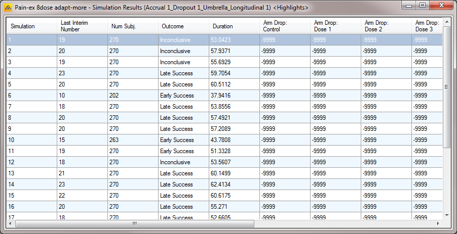
Detailed Per Simulation Results
After simulation has completed and simulation results have been loaded, the user may examine detailed results for any scenario with simulations output in the table by double-clicking on the appropriate row. A separate window pops up and displays the results for each individual simulation. This is a “prettier” view of the contents of the “simulations.csv” file, which is described below. The simulations results are partitioned into the same results groupings as the summary results. These can be accessed from the “right click” menu, along with opening the results folder, opening the weeks file for a particular simulation and opening the simulated patients file for a particular simulation (where a “weeks” file or a “patients” file has been output).
Output Files
Instead of viewing simulation output on the Simulation tab within FACTS, the output is all contained within easily accessible files saved the the user’s local machine. FACTS stores the results of simulations as ‘.csv’ files under a Results folder. For each row in the simulations table, there is a folder named by the profiles that make up the scenario, which contains the corresponding ‘.csv’ files.
These files can be opened using Microsoft Excel or any text editor. Excel, and many other apps, takes out a file lock on any file it has open, while a FACTS results file is open in another piece of software it cannot be deleted or modified by FACTS. The most common cause for an error to be reported when simulating trials in FACTS is because the user has one of the previous results files is still open in Excel.
In the scenario directory there are the following types of results file:
Summary.csv Contains a single row of data that summarizes the simulation results. This is the source of the shown on the simulations tab.
Summary_freq_bocf_NNNNN.csv, Continuous only. Summary_freq_locf_NNNN.csv, Summary_freq_ignore_NNNN.csv, Summary_freq_fail_NNNNN.csv, Dichotomous only. Contains a single row of data that that summarizes the frequentist analysis of the simulations. A file is output for each of the different methods for dealing with missing data that are selected on the Frequentist Analysis tab: BOCF if the baseline score is being simulated, LOCF and “ignore” (referred to as PP (Per-Protocol) in the GUI).
Simulations.csv Contains one row per simulation describing the final state of each simulation for every trial simulated.
Simulations_freq.csv Contains one row per simulation describing the frequentist analysis of the final state of each simulation for every trial simulated.
PatientsNNNNN.csv Contains one row per patient in a simulation, where NNNNN is the number of the simulation. By default this file is written out only for the first simulation, but this can be changed on the simulations tab.
WeeksNNNNN.csv Contains one row for each cohort during a simulation where NNN is the number of the simulation. By default this file is written only for the first 100 simulations, but this can be changed via the simulation tab. The values in the last row of the cohorts file will be the same as the final values for that simulation in the simulations file.
weeks_freq_bocf_NNNNN.csv, Continuous only. weeks_freq_locf_NNNN.csv, weeks_freq_ignore_NNNN.csv, weeks_freq_fail_NNNNN.csv, Dichotomous only. Contains one row for each interim during a simulation where NNNNN is the number of the simulation. A file is output for each simulation for which a frequentist “weeks file” is to be output, and for each of the different methods for dealing with missing data that are applicable.
Contents of summary.csv
The first line is a header line, starting with a ‘#’, containing the FACTS GUI version number, the name of the FACTS file, the name of the scenario, and the time stamp of the start of the simulation.
The second line is a header line, starting with a ‘#’, containing the following column headings.
| Column Title | Number of columns | Description |
|---|---|---|
| Project | 1 | The name of the facts file |
| Scenario | 1 | The name of the scenario |
| Timestamp | 1 | The time the simulations were run |
| Version | 1 | The version of FACTS that was used to run the simulations |
| NSim | 1 | The number of simulation run. |
| Random Number Seed | 1 | The random number seed |
| No. Subj | 1 | The mean, over the simulations, of the total number of subjects recruited in the trial. |
| SE Subj. | 1 | The standard error of the total number of subjects recruited into the trials. |
| No.Subj 80%ile | 1 | The 80th percentile, over the simulations, of the total number of subjects recruited in the trial. |
| Ppn Overall Success | 1 | The proportion of simulations that were successful (P(ES) + P(LS)) |
| Ppn Overall Futility | 1 | The proportion of simulations that were futile (P(EF) + P(LF)) |
| P(ES) | 1 | The proportion of simulations that stopped early for success. |
| P(LS) | 1 | The proportion of simulations that did not stop early, and were successful on final evaluation. |
| P(LF) | 1 | The proportion of simulations that did not stop early, and were futile on final evaluation. |
| P(EF) | 1 | The proportion of simulations that stopped early for futility. |
| SFFF | 1 | The proportion of simulations that stopped early for success, but at final analysis were futile (Success-Futility ‘flip-flops’). |
| FSFF | 1 | The proportion of simulations that stopped early for futility, but at final analysis were successful (Futility- Success ‘flip-flops’). |
| Undec. | 1 | The proportion of simulations that did not stop early, and met neither the success or futility final evaluation criteria and hence are counted as ‘undecided’. |
| Unused | 3 | Three unused columns for other outcome types. |
| Early Success Time | 1 | This is the mean early decision time (over the simulations stopped early for success), it is the time from the start of the trial to the interim where early success was declared. It does not include the subsequent follow up time. |
| Mean Alloc <Dose> | D | The mean (over the simulations) of the number of subjects allocated to each treatment arm. |
| SE Alloc <Dose> | D | The standard error (over the simulations) of the number of subjects allocated to each treatment arm. |
| Mean Resp <Dose> | D | The mean of the estimates of response of each treatment arm. |
| SE Resp <Dose> | D | The standard error, over the simulations, of the estimate of response of each treatment arm. |
| Mean Sigma | 1 | The mean of the estimate of sigma – the average standard deviation of the dose response |
| SE Mean Sigma | 1 | The standard error of the estimate of sigma – the average standard deviation of the dose response |
| True Mean resp <Dose> | D | The true response for each treatment arm used when sampling the simulated subject responses. |
| True SD resp <Dose> | D | The true SD of the response for each treatment arm of the simulated subject responses |
| Mean Longmod Resp: <Dose> <Visit> | D*V | These are only calculated and written out if the Time Course Hierarchical or ITP longitudinal models are being used. This is the mean (over the simulations) of the estimate of the mean response for a particular dose at a particular visit. |
| SE Mean Longmod Resp: <Dose> <Visit> | D*V | This is the standard error (over the simulations) of the longitudinal model estimate of the response at intermediate visits (see above) |
| Mean Complete <Dose> | D | The mean number of completers for each treatment arm |
| Mean Complete Info <Dose> | D | The mean number of complete information (as specified by the interim information type on the Interims tab) for each treatment arm |
| No .Dropouts <Dose> <Visit> | D*V | The mean number of dropouts per treatment arm per visit |
| Mean Beta | 1 | The mean of the estimates of the coefficient of baseline adjustment |
| SE beta | 1 | The standard error of the estimates of the coefficient of baseline adjustment |
| Mean Baseline | 1 | The mean of the estimate of the mean of the baseline score |
| SE Mean Baseline | 1 | The standard error of the estimate of the mean of the baseline score |
| SD Baseline | 1 | The mean of the estimate of the SD of the baseline score |
| SE SD Baseline | 1 | The standard error of the estimate of the SD of the baseline score |
| True Mean Baseline | 1 | The true mean of the baseline score (accounting for possible truncation) |
| True SD Baseline | 1 | The true SD of the baseline score (accounting for possible truncation) |
| BAC Mean | 1 | If a hierarchical prior for Control is being used this is the mean (over the simulations) of the posterior estimate of the mean of the Bayesian Augmented Control (Hierarchical Prior) distribution of mean control responses. |
| SE of BAC Mean | 1 | If a hierarchical prior for Control is being used this is the standard error (over the simulations) of the posterior estimate of the mean of the Bayesian Augmented Control (Hierarchical Prior) distribution of mean control responses. |
| BAC Tau | 1 | If a hierarchical prior for Control is being used this is the mean (over the simulations) of the posterior estimate of the SD of the Bayesian Augmented Control (Hierarchical Prior) distribution of mean control responses. |
| SE of BAC Tau | 1 | If a hierarchical prior for Control is being used this is the standard error (over the simulations) of the posterior estimate of the SD of the Bayesian Augmented Control (Hierarchical Prior) distribution of mean control responses. |
| BAAC Mean | 1 | If a hierarchical prior for Active Comparator is being used this is the mean (over the simulations) of the posterior estimate of the mean of the Bayesian Augmented Active Comparator (Hierarchical Prior) distribution of mean active comparator responses. |
| SE of BAAC Mean | 1 | If a hierarchical prior for Active Comparator is being used this is the standard error (over the simulations) of the posterior estimate of the mean of the Bayesian Augmented Active Comparator (Hierarchical Prior) distribution of mean control responses. |
| BAAC Tau | 1 | If a hierarchical prior for Active Comparator is being used this is the mean (over the simulations) of the posterior estimate of the SD of the Bayesian Augmented Active Comparator (Hierarchical Prior) distribution of mean active comparator responses. |
| SE of BAAC Tau | 1 | If a hierarchical prior for Active Comparator is being used this is the standard error (over the simulations) of the posterior estimate of the SD of the Bayesian Augmented Active Comparator (Hierarchical Prior) distribution of mean active comparator responses. |
| Mean Duration | 1 | The mean, over the simulations, of the overall duration of the trials, from first person first visit, to last person last visit. |
| Ppn Arms Dropped <Dose> | D | The proportion of the simulations in which each arm was dropped. These will be zero if arm dropping is not selected as the means of adaptive allocation. |
| Mean LPFV time | 1 | The mean, over the simulations, of the accrual period of the trials, from first person first visit, to last person first visit (LPFV). |
| Ppn Correct Arm | 1 | The proportion of the simulations where the correct arm has been selected, where an arm is deemed “correct” based on whether it was marked as “Should Succeed” for the relevant scenario on the VSR tab. |
| Ppn Incorrect Arm | 1 | The proportion of the simulations where the incorrect correct arm has been selected, where an arm is deemed “incorrect” based on whether it wasn’t marked as “Should Succeed” for the relevant scenario on the VSR tab. |
| QOI Columns | See next section. |
| Column Title | Number of columns | Description |
|---|---|---|
| Project | 1 | The name of the facts file |
| Scenario | 1 | The name of the scenario |
| Timestamp | 1 | The time the simulations were run |
| Version | 1 | The version of FACTS that was used to run the simulations |
| NSim | 1 | The number of simulation run. |
| Random Number Seed | 1 | The random number seed |
| No. Subj | 1 | The mean, over the simulations, of the total number of subjects recruited in the trial. |
| SE Subj. | 1 | The standard error of the total number of subjects recruited into the trials. |
| No.Subj 80%ile | 1 | The 80th percentile, over the simulations, of the total number of subjects recruited in the trial. |
| Ppn Overall Success | 1 | The proportion of simulations that were successful (P(ES) + P(LS)) |
| Ppn Overall Futility | 1 | The proportion of simulations that were futile (P(EF) + P(LF)) |
| P(ES) | 1 | The proportion of simulations that stopped early for success. |
| P(LS) | 1 | The proportion of simulations that did not stop early, and were successful on final evaluation. |
| P(LF) | 1 | The proportion of simulations that did not stop early, and were futile on final evaluation. |
| P(EF) | 1 | The proportion of simulations that stopped early for futility. |
| SFFF | 1 | The proportion of simulations that stopped early for success, but at final analysis were futile (Success-Futility ‘flip-flops’). |
| FSFF | 1 | The proportion of simulations that stopped early for futility, but at final analysis were successful (Futility- Success ‘flip-flops’). |
| Undec. | 1 | The proportion of simulations that did not stop early, and met neither the success or futility final evaluation criteria and hence are counted as ‘undecided’. |
| Unused | 3 | Three unused columns for other outcome types. |
| Early Success Time | 1 | This is the mean early decision time (over the simulations stopped early for success), it is the time from the start of the trial to the interim where early success was declared. It does not include the subsequent follow up time. |
| Mean Alloc <Dose> | D | The mean (over the simulations) of the number of subjects allocated to each treatment arm. |
| SE Alloc <Dose> | D | The standard error (over the simulations) of the number of subjects allocated to each treatment arm. |
| Mean Resp <Dose> | D | The mean of the estimates of response of each treatment arm. |
| SE Resp <Dose> | D | The standard error, over the simulations, of the estimate of response of each treatment arm. |
| True Mean resp <Dose> | D | The true response for each treatment arm used when sampling the simulated subject responses. |
| Mean Longmod Resp: <Dose> <Visit> | D*V | These are only calculated and written out if the Time Course Hierarchical or ITP longitudinal models are being used. This is the mean (over the simulations) of the estimate of the mean response for a particular dose at a particular visit. |
| SE Mean Longmod Resp: <Dose> <Visit> | D*V | This is the standard error (over the simulations) of the longitudinal model estimate of the response at intermediate visits (see above) |
| Mean Complete <Dose> | D | The mean number of completers for each treatment arm |
| Mean Complete Info <Dose> | D | The mean number of complete information (as specified by the interim information type on the Interims tab) for each treatment arm |
| No .Dropouts <Dose> <Visit> | D*V | The mean number of dropouts per treatment arm per visit |
| BAC Mean | 1 | If a hierarchical prior for Control is being used this is the mean (over the simulations) of the posterior estimate of the mean of the Bayesian Augmented Control (Hierarchical Prior) distribution of mean control responses. |
| SE of BAC Mean | 1 | If a hierarchical prior for Control is being used this is the standard error (over the simulations) of the posterior estimate of the mean of the Bayesian Augmented Control (Hierarchical Prior) distribution of mean control responses. |
| BAC Tau | 1 | If a hierarchical prior for Control is being used this is the mean (over the simulations) of the posterior estimate of the SD of the Bayesian Augmented Control (Hierarchical Prior) distribution of mean control responses. |
| SE of BAC Tau | 1 | If a hierarchical prior for Control is being used this is the standard error (over the simulations) of the posterior estimate of the SD of the Bayesian Augmented Control (Hierarchical Prior) distribution of mean control responses. |
| BAAC Mean | 1 | If a hierarchical prior for Active Comparator is being used this is the mean (over the simulations) of the posterior estimate of the mean of the Bayesian Augmented Active Comparator (Hierarchical Prior) distribution of mean active comparator responses. |
| SE of BAAC Mean | 1 | If a hierarchical prior for Active Comparator is being used this is the standard error (over the simulations) of the posterior estimate of the mean of the Bayesian Augmented Active Comparator (Hierarchical Prior) distribution of mean control responses. |
| BAAC Tau | 1 | If a hierarchical prior for Active Comparator is being used this is the mean (over the simulations) of the posterior estimate of the SD of the Bayesian Augmented Active Comparator (Hierarchical Prior) distribution of mean active comparator responses. |
| SE of BAAC Tau | 1 | If a hierarchical prior for Active Comparator is being used this is the standard error (over the simulations) of the posterior estimate of the SD of the Bayesian Augmented Active Comparator (Hierarchical Prior) distribution of mean active comparator responses. |
| Mean Duration | 1 | The mean, over the simulations, of the overall duration of the trials, from first person first visit, to last person last visit. |
| Ppn Arms Dropped <Dose> | D | The proportion of the simulations in which each arm was dropped. These will be zero if arm dropping is not selected as the means of adaptive allocation. |
| Mean LPFV time | 1 | The mean, over the simulations, of the accrual period of the trials, from first person first visit, to last person first visit (LPFV). |
| Ppn Correct Arm | 1 | The proportion of the simulations where the correct arm has been selected, where an arm is deemed “correct” based on whether it was marked as “Should Succeed” for the relevant scenario on the VSR tab. |
| Ppn Incorrect Arm | 1 | The proportion of the simulations where the incorrect correct arm has been selected, where an arm is deemed “incorrect” based on whether it wasn’t marked as “Should Succeed” for the relevant scenario on the VSR tab. |
| QOI Columns | See next section. |
QOI Columns
The QOI columns depend on the QOIs that have been defined for this design. The columns in the following order:
| Statistic | Description |
|---|---|
| Posterior Probabilities | The summary file contains the mean (over the simulations) of the posterior probability for each dose. |
| Predictive Probabilities | The summary file contains the mean (over the simulations) of the predictive probability for each dose. |
| P-Values | The summary file contains the mean (over the simulations) of the p-value for each dose. |
| Target Probabilities | The summary file contains the proportion of times (over the simulations) each dose had the greatest probability of being the target. |
| Decision QOIs | The summary file contains the mean (over the simulations) of the final value of the decision QOI at the target. |
Contents of Summary_freq_{missingnessType}.csv
There is a frequentist summary file for each type of treatment of missing values.
The first line is a header line, starting with a ‘#’, containing the FACTS GUI version number, the name of the FACTS file, the name of the scenario, and the time stamp of the start of the simulation.
The second line is a header line, starting with a ‘#’, containing the following column headings.
| Column Title | Number of columns | Description |
|---|---|---|
| Mean Theta <Dose> | D | The mean response per dose. |
| SE Theta <Dose> | D | The standard error of the response per dose |
| Mean Beta (b aseline) | 1 | The mean of the estimate of the baseline coefficient. |
| SE Mean Beta (b aseline) | 1 | The standard error of the estimate of the baseline coefficient |
| Ppn Signif | 1 | The proportion of simulations where at least one of the unadjusted p-values is less than the user specified one-sided alpha. |
| Ppn Signif <Dose> | D | For each treatment arm, the proportion of simulations where the unadjusted p-value is less than the user specified one-sided alpha. The marginal probability of significance per dose (using unadjusted p-values. |
| Bias <Dose> | D | The difference between the estimated mean response and the true (simulated) mean response per dose |
| Coverage <Dose> | D | The proportion of simulations where the unadjusted confidence interval for the response contains the true mean response used to simulate subject responses. |
| Ppn Signif Dunnett | 1 | The proportion of simulations where at least one of the Dunnett adjusted p-values is less than the user specified one-sided alpha. |
| Ppn Signif Dunnett <Dose> | D | For each treatment arm, the proportion of simulations where the Dunnett adjusted p-value is less than the user specified one-sided alpha. |
| Coverage Dunnett <Dose> | D | The proportion of simulations where the Dunnett adjusted confidence interval contains the true mean response used to simulate subjects responses. |
| Ppn Signif Bonf | 1 | The proportion of simulations where at least one of the Bonferroni adjusted p-values is less than the user specified one-sided alpha. |
| Ppn Signif Bonf <Dose> | D | For each treatment arm, the proportion of simulations where the Bonferroni adjusted p-value is less than the user specified one-sided alpha. |
| Coverage Bonf <Dose> | D | The proportion of simulations where the Bonferroni adjusted confidence interval contains the true mean response used to simulate subjects responses. |
| Ppn Signif Trend | 1 | The proportion of simulations where the trend test p-value is less than the user specified one-sided alpha. |
| Column Title | Number of columns | Description | |
|---|---|---|---|
| Mean Theta <Dose> | D | The mean response per dose. | |
| SE Theta <Dose> | D | The standard error of the response per dose | |
| Ppn Signif | 1 | The proportion of simulations where at least one of the unadjusted p-values is less than the user specified one-sided alpha. | |
| Ppn Signif <Dose> | D | For each treatment arm, the proportion of | simulations where the unadjusted p-value is | less than the user specified one-sided alpha. | | The marginal probability of significance per | dose (using unadjusted p-values). | |
| Bias <Dose> | D | The difference between the estimated mean response and the true (simulated) mean response per dose | |
| Coverage <Dose> | D | The proportion of simulations where the unadjusted confidence interval for the response contains the true mean response used to simulate subject responses. | |
| Ppn Signif Dunnett | 1 | The proportion of simulations where at least one of the Dunnett adjusted p-values is less than the user specified one-sided alpha. | |
| Ppn Signif Dunnett <Dose> | D | For each treatment arm, the proportion of simulations where the Dunnett adjusted p-value is less than the user specified one-sided alpha. | |
| Coverage Dunnett <Dose> | D | The proportion of simulations where the Dunnett adjusted confidence interval contains the true mean response used to simulate subjects responses. | |
| Ppn Signif Bonf | 1 | The proportion of simulations where at least one of the Bonferroni adjusted p-values is less than the user specified one-sided alpha. | |
| Ppn Signif Bonf <Dose> | D | For each treatment arm, the proportion of simulations where the Bonferroni adjusted p-value is less than the user specified one-sided alpha. | |
| Coverage Bonf <Dose> | D | The proportion of simulations where the Bonferroni adjusted confidence interval contains the true mean response used to simulate subjects responses. | |
| Ppn Signif Trend | 1 | The proportion of simulations where the trend test p-value is less than the user specified one-sided alpha. | |
Contents of simulations.csv and weeksNNNNN.csv
The simulations.csv file holds the FACTS summary of the final analysis for each simulation (one per row).
The weeksNNNNN.csv file holds the FACTS summary of every analysis for the NNNNNth simulation. It contains a row for each interim in the trial and a row for the final analysis (Interim number 999).
The final analysis occurs after all the planned data is collected. If the trial does not stop early, the final analysis occurs after full follow-up for all subjects. If the trial does stop early at an interim analysis, then the timing of the final analysis depends on the status of the check boxes on the Interims tab. If follow-up is collected after the particular interim decision, then an analysis after full follow-up of the subjects recruited up to the point of the interim when the stopping decision was taken. If there is no follow-up intended after the interim analysis decision, then the final analysis occurs immediately (at the same time as the interim analysis), and the final analysis criteria are checked.
The first line is a header line, starting with a ‘#’, containing the FACTS GUI version number, the name of the FACTS file, the name of the scenario, and the time stamp of the start of the simulation.
The second line is a header line, starting with a ‘#’, containing the following column headings.
Most of the columns are common to the two file types, but the weeks file does not contain columns for the ‘final’ values of the evaluation criteria.
| Column Title | Number of columns | In simulations file | In weeks file | Description |
|---|---|---|---|---|
| # Weeks (Duration) | 1 | ✔ | The week of the analysis | |
| #Sim | 1 | ✔ | The number of the simulation. | |
| Random Number Seed | 1 | ✔ | ✔ | Base random number seed. |
| LastInterim | 1 | ✔ | The index of the last interim performed the index of the interim immediately before the final interim (index ‘999’). Note this is not necessarily the interim when the trial stopped if the design includes follow-up after stopping. | |
| #Subjects | 1 | ✔ | ✔ | The number of subjects recruited in the simulation. |
| Outcome | 1 | ✔ | ✔ | A flag categorizing final study outcome: 1 = Early success 2 = Late success 3 = Late futility 4 = Early futility 5 = Success to futility flip-flop 6 = Futility to success flip-flop 7 = Inconclusive |
| Early Success Time | 1 | ✔ | ✔ | This is the time to the early success decision (-9999 if there was no early success decision). The from the start of the trial to the interim where the early success conditions were first met. It does not include the subsequent follow up time. |
| Alloc <Dose> | D | ✔ | ✔ | The number of subjects allocated to each arm. |
| Pr(Alloc) <Dose> | D | ✔ | ✔ | The probability of allocation to the different arms following the interim. |
| Mean resp <Dose> | D | ✔ | ✔ | The estimated response of each treatment arm. |
| SD Mean resp <Dose> | D | ✔ | ✔ | The standard deviation of the estimate of response of each treatment arm. |
| True Mean resp <Dose> | D | ✔ | ✔ | The true mean response of each treatment arm for this simulation. |
| True SD resp <Dose> | D | ✔ | ✔ | The true SD of the response of each treatment arm for this simulation |
| Sigma | 1 | ✔ | ✔ | The pooled estimate of the SD of the response across all the treatment arms |
| SD_Sigma | 1 | ✔ | ✔ | The SD of the pooled estimate of the SD of the response across all the treatment arms |
| Beta | 1 | ✔ | ✔ | The estimate of ‘Beta’ the baseline adjustment coefficient, if baseline adjustment is being used. |
| SD_Beta | 1 | ✔ | ✔ | The SD of the estimate of ‘Beta’ the baseline adjustment coefficient. |
| Mean Baseline | 1 | ✔ | ✔ | The estimate of the mean baseline score. |
| SE Mean Baseline | 1 | ✔ | ✔ | The standard error of the estimate of the mean baseline score. |
| SD Baseline | 1 | ✔ | ✔ | The estimate of the SD of the baseline score. |
| True Mean Baseline | 1 | ✔ | ✔ | The true mean of the simulated baseline score |
| True SD Baseline | 1 | ✔ | ✔ | The true SD of the simulated baseline score |
| Mean Raw Response <Dose> | D | ✔ | ✔ | The observed mean response on each treatment arm (unadjusted by any modeling). |
| SE Mean Raw Response <Dose> | D | ✔ | ✔ | The SE of the estimate of the mean raw response on each dose. |
| Complete <Dose> | D | ✔ | ✔ | The number of completed subjects on each treatment arm at the time of the analysis. |
| Complete Information <Dose> | D | ✔ | ✔ | The number of subject who count as complete for the purposes of timing interims – whether complete or opportunity to complete and at which visit is as defined on the Interims tab. If interims are by enrolment then CompleteInformation is the number of subjects that have completed – final endpoint data is available. |
| #Dropouts <Dose> <Visit> | D * V | ✔ | ✔ | The number of subjects dropped out on each treatment arm and each visit. |
| DR Param <Param> | 10 | ✔ | ✔ | The estimate of the mean value of each of the response model parameters. The response models require up to 10 parameters, most less. The model parameters are labeled \(\alpha_1\), \(\alpha_2\), .. the subscripts corresponding to the index “<Param>”. |
| Sd DR Param <Param> | 4 | ✔ | ✔ | The standard deviation of the estimate of the mean value of the corresponding response model parameter. |
| Longmod_ <Model> <Parameter> <Visit> | LM * LMP * V | ✔ | ✔ | The estimate of the mean value of each of the longitudinal model parameters. The number of models depends on the number of “model instances” the user has specified. For linear regression the parameters reported are: - Alpha – per visit – the mean estimate of the constant offset in the change in response from this visit to the final visit - Beta – per visit – the mean estimate of the coefficient of change in response from this visit to the final visit - Lambda – per visit – the mean estimate of the SD of the residual error term in the predicted final visit response based on the response at this visit. For time course hierarchical the parameters reported are: - Alpha – per visit – the mean estimate of the exponential coefficient of the proportion of the dose response and per-subject response seen at this visit.. - Lambda – per visit – the mean estimate of the SD of the residual error term in the predicted final visit response based on the response at this visit. - Tau – the mean estimate of the SD of the per subject random effect For ITP the parameters are: - K – per model – the mean estimate of the ITP shape parameter - Tau – per model - the mean estimate of the SD of the per subject random effect - Lambda – per model – the mean estimate of the Sd of the residual error. - Omega – per treatment arm – the mean estimate of the mean treatment arm effect. For LOCF & Kernel Density there are no estimated parameters. |
| Longmod Resp: <Dose> <Visit> | D * V | ✔ | ✔ | These are only calculated and written out if the Time Course Hierarchical or ITP longitudinal models are being used. This is the mean response for a particular dose at a particular visit. |
| BAC Mean | 1 | ✔ | ✔ | This is the posterior estimate of the mean of the Bayesian Augmented Control (Hierarchical Prior) distribution of mean control responses. |
| BAC Mean SD | 1 | ✔ | ✔ | This is the SD of the posterior estimate of the mean of the Bayesian Augmented Control (Hierarchical Prior) distribution of mean control responses. |
| BAC Tau | 1 | ✔ | ✔ | This is the posterior estimate of the SD of the Bayesian Augmented Control (Hierarchical Prior) distribution of mean control responses. |
| BAC Tau SD | 1 | ✔ | ✔ | This is the SD of the posterior estimate of the SD of the Bayesian Augmented Control (Hierarchical Prior) distribution of mean control responses. |
| BAAC Mean | 1 | ✔ | ✔ | This is the posterior estimate of the mean of the Bayesian Augmented Active Comparator (Hierarchical Prior) distribution of mean active comparator responses. |
| BAAC Mean SD | 1 | ✔ | ✔ | This is the SD of the posterior estimate of the mean of the Bayesian Augmented Active Comparator (Hierarchical Prior) distribution of mean comparator responses. |
| BAAC Tau | 1 | ✔ | ✔ | This is the posterior estimate of the SD of the Bayesian Augmented Active Comparator (Hierarchical Prior) distribution of mean active comparator responses. |
| BAAC Tau SD | 1 | ✔ | ✔ | This is the SD of the posterior estimate of the SD of the Bayesian Augmented Active Comparator (Hierarchical Prior) distribution of mean active comparator responses. |
| Duration | 1 | ✔ | ✔ | The time in weeks to the analysis shown. |
| Arm Drop Time <Dose> | D | ✔ | ✔ | For each treatment arm, the time in weeks when it was decided to drop the arm. |
| LPFV | 1 | ✔ | ✔ | The time in weeks to the last patient first visit. |
| QOI Columns | ✔ | ✔ | See next section. |
| Column Title | Number of columns | In simulations file | In weeks file | Description |
|---|---|---|---|---|
| # Weeks (Duration) | 1 | ✔ | The week of the analysis | |
| #Sim | 1 | ✔ | The number of the simulation | |
| LastInterim | 1 | ✔ | The index of the last interim performed the index of the interim immediately before the final interim (index ‘999’). Note this is not necessarily the interim when the trial stopped if the design includes follow-up after stopping | |
| #Subjects | 1 | ✔ | ✔ | The number of subjects recruited in the simulation |
| Outcome | 1 | ✔ | ✔ | A flag categorizing final study outcome: 1 = Early success 2 = Late success 3 = Late futility 4 = Early futility 5 = Success to futility flip-flop 6 = Futility to success flip-flop 7 = Inconclusive |
| Early Success Time | 1 | ✔ | ✔ | This is the time to the early success decision (-9999 if there was no early success decision). The from the start of the trial to the interim where the early success conditions were first met. It does not include the subsequent follow up time |
| Alloc <Dose> | D | ✔ | ✔ | The number of subjects allocated to each arm |
| Pr(Alloc) <Dose> | D | ✔ | ✔ | The probability of allocation to the different arms following the interim |
| Mean resp <Dose> | D | ✔ | ✔ | The estimated response of each treatment arm |
| SD resp <Dose> | D | ✔ | ✔ | The standard deviation of the estimate of response of each treatment arm |
| Mean resp (lower CI) <Dose> | D | ✔ | ✔ | The lower bound of the 95% Credible Interval of the estimate of response for each treatment arm |
| Mean resp (upper CI) <Dose> | D | ✔ | ✔ | The upper bound of the 95% Credible Interval of the estimate of response for each treatment arm |
| True Mean resp <Dose> | D | ✔ | ✔ | The true mean response of each treatment arm for this simulation |
| Mean Raw Response <Dose> | D | ✔ | ✔ | The observed rate of response on each treatment arm (unadjusted by any modeling) |
| Complete <Dose> | D | ✔ | ✔ | The number of completed subjects on each treatment arm at the time of the analysis |
| Complete Information <Dose> | D | ✔ | ✔ | The number of subjects that have achieved the information criteria as specified on the Interims tab. May be the number enrolled, complete, or with the opportunity to complete. If complete or opportunity to complete, then the visit that should be complete is also specified. |
| #Dropouts <Dose> <Visit> | D * V | ✔ | ✔ | The number of subjects dropped out on each treatment arm and each visit |
| DR Param <Param> | 4 | ✔ | ✔ | The estimate of the mean value of each of the response model parameters. The response models require up to 4 parameters, some less. The model parameters are labeled \(\alpha_1\), \(\alpha_2\), .. the subscripts corresponding to the column their value appears in here |
| Sd DR Param <Param> | 4 | ✔ | ✔ | The standard deviation of the estimate of the mean value of the corresponding response model parameter |
| Longmod_ <Model> <Parameter> <Visit> | LM * LMP * V | ✔ | ✔ | The estimate of the mean value of each of the longitudinal model parameters. The number of models depends on the number of “model instances” the user has specified. Each value is reported per visit unless otherwise stated. For Beta-Binomial the parameters reported are: • Alpha0 & Beta 0 – The beta binomial alpha & beta parameters for the probability that the final result will be 1 if the result at the visit is 0 • Prob01 – the mean probability of the Beta(Alpha0, Beta0) – the probability of 1 being the final result if the result at the visit is 0 • Alpha1 & Beta 1 – The beta binomial alpha & beta parameters for the probability that the final result will be 1 if the result at the visit is 1 • Prob11 – the mean probability of the Beta(Alpha1, Beta1) – the probability of 1 being the final result if the result at the visit is 1 For logistic regression the parameters reported are: • Prob11 – the probability of 1 being the final result if the result at the visit is 1and • Prob01 – the probability of 1 being the final result if the result at the visit is 0 For restricted Markov the parameters reported are: • Alpha0 – Alpha for state 0 • AlphaS – Alpha for stable state • Alpha1 – Alpha for state 1 • Prob0 – Transition probability to state 0 • ProbS – Probability of remaining stable • Prob1 – Transition probability to state 1 (values are for the transition to the next visit, so thre are no values for the final visit) If using a dichotomized continuous response, these columns will be for the selected continuous longitudinal model: For linear regression the parameters reported are: • Alpha – the mean estimate of the constant offset in the change in response from this visit to the final visit • Beta – the mean estimate of the coefficient of change in response from this visit to the final visit • Lambda – the mean estimate of the SD of the residual error term in the predicted final visit response based on the response at this visit. For ITP the parameters are: • K – single value per model – the mean estimate of the ITP shape parameter • Tau – single value per model - the mean estimate of the SD of the per subject random effect • Lambda – single value per model – the mean estimate of the Sd of the residual error. • Omega – per treatment arm not visit – the mean estimate of the mean treatment arm effect. For LOCF & Kernel Density there are no estimated parameters. |
| Longmod Resp: <Dose> <Visit> | D * V | ✔ | ✔ | These are only calculated and written out if the ITP longitudinal model is being used for a dichotomized continuous endpoint. This is the mean response for a particular dose at a particular visit. |
| BAC Mean | 1 | ✔ | ✔ | This is the posterior estimate of the mean of the Bayesian Augmented Control (Hierarchical Prior) distribution of mean control responses |
| BAC Mean SD | 1 | ✔ | ✔ | This is the SD of the posterior estimate of the mean of the Bayesian Augmented Control (Hierarchical Prior) distribution of mean control responses |
| BAC Tau | 1 | ✔ | ✔ | This is the posterior estimate of the SD of the Bayesian Augmented Control (Hierarchical Prior) distribution of mean control responses |
| BAC Tau SD | 1 | ✔ | ✔ | This is the SD of the posterior estimate of the SD of the Bayesian Augmented Control (Hierarchical Prior) distribution of mean control responses |
| BAAC Mean | 1 | ✔ | ✔ | This is the posterior estimate of the mean of the Bayesian Augmented Active Comparator (Hierarchical Prior) distribution of mean active comparator responses |
| BAAC Mean SD | 1 | ✔ | ✔ | This is the SD of the posterior estimate of the mean of the Bayesian Augmented Active Comparator (Hierarchical Prior) distribution of mean comparator responses |
| BAAC Tau | 1 | ✔ | ✔ | This is the posterior estimate of the SD of the Bayesian Augmented Active Comparator (Hierarchical Prior) distribution of mean active comparator responses |
| BAAC Tau SD | 1 | ✔ | ✔ | This is the SD of the posterior estimate of the SD of the Bayesian Augmented Active Comparator (Hierarchical Prior) distribution of mean active comparator responses |
| Duration | 1 | ✔ | ✔ | The time in weeks to the analysis shown |
| Arm Drop Time <Dose> | D | ✔ | ✔ | For each treatment arm, the time in weeks when it was decided to drop the arm |
| LPFV | 1 | ✔ | ✔ | The time in weeks to the last patient first visit |
| QOI Columns | ✔ | ✔ | See next section. |
QOI Columns
The QOI columns depend on the QOIs that have been defined for this design. The columns are grouped in the following order:
| QOI Type | Description |
|---|---|
| Posterior Probabilities | The posterior probability for each QOI for each dose. |
| Predictive Probabilities | The predictive probability for each QOI for each dose. |
| P-Values | The p-value for each QOI for each dose. |
| Target Probabilities | The probability of being the target for each QOI for each dose. |
| Decision QOIs | The value of the decision QOI at the target. |
| Success Futile | A flag for each QOI decision criteria indicating if the decision QOI was evaluated and compared to a threshold at the interim (weeks file) or final analysis (simulation file). The flag value is -1 if the decision QOI was not evaluated, 0 if it did not meet the threshold and 1 if it did. |
| Success / Futile Combined | Flags indicating if the interim or final analysis determined success or futility taking all the factors defined for Success/Futility into account: 0 if the conditions were not met, 1 it the conditions were met. If success and futility conditions have been defined that are not mutually exclusive and both sets of combined conditions are met, FACTS will pick one of the outcomes as met but not the other. In order to discourage defining Success and Futility rules that can both be true FACTS does not guarantee which outcome will be selected. |
Contents of Simulations_freq_{missingnessType}.csv, Weeks_freq_{missingnessType}.csv
These file contain the frequentist results after an interim analysis (weeks file) or final analysis (simulations file), apart for the first column, the columns are the same in the two types of file, and the same across the different methods for treating missing data.
| Column | Number of columns | Description |
|---|---|---|
| # Trial | 1 | The number of the simulation (simulations_freq_…csv only) |
| # Weeks | 1 | The week of the interim (weeks_freq_…csv only) |
| Theta | D | Unadjusted estimate of response per treatment arm |
| Theta SD | D | The SD of the estimate of response per treatment arm |
| Trt Effect | D | The relative size of the treatment effect compared to control per arm (treatment effect for control is always 0). The direction of the comparison takes into account whether a response represents a subject’s condition improving or worsening, so that a positive treatment effect shows the response on the dose is better than on control. |
| t-Stat | D | The t-test statistic per treatment arm (for control this is always 0) |
| p-Value | D | The unadjusted t-test p-value per arm (for control this is always 0) |
| lower CI | D | The unadjusted lower bound of the alpha confidence interval of the estimated treatment effect per treatment arm (for control this is always 0). |
| upper CI | D | The unadjusted upper bound of the alpha confidence interval of the estimated treatment effect per treatment arm (for control this is always 0). |
| Min p-Value | 1 | The smallest of the t-test p-values |
| p-Value Dunnett | D | The Dunnett adjusted t-test p-value per arm (for control this is always 0). |
| lower CI Dunnett | D | The Dunnett adjusted lower bound of the alpha confidence interval of the estimated treatment effect (for control this is always 0). |
| upper CI Dunnett | D | The Dunnett adjusted upper bound of the alpha confidence interval of the estimated treatment effect (for control this is always 0). |
| Min p-Value Dunnett | 1 | The smallest of the Dunnett adjusted p-values. |
| p-Value Bonf | D | The Bonferroni adjusted t-test p-value per arm. |
| lower-CI Bonf | D | The Bonferroni adjusted lower bound of the alpha confidence interval of the estimated treatment effect (for control this is always 0). |
| upper-CI Bonf | D | The Bonferroni adjusted upper bound of the alpha confidence interval of the estimated treatment effect (for control this is always 0). |
| Min p-Value Bonf | 1 | The smallest of the Bonferroni adjusted t-test value per arm. |
| t-Stat trend | 1 | The t statistic from the trend test. |
| p-Value trend | 1 | The p-value from the trend test. |
Contents of PatientsNNNNN.csv
| Column | Number of columns | Description |
|---|---|---|
| Subject | 1 | The subject id number, starting at 1. |
| Region | 1 | Which region the subject was recruited in. |
| Date | 1 | The date, in weeks from the start of the trial, of the subject’s baseline visit and randomization. |
| Dose | 1 | The index number (1, …) of the treatment arm the subject belongs to. |
| LastVisit# | 1 | The index of the last visit for which the subjects data was collected, if the subject did not complete all of its visits it could be because they dropped-out, the subject’s treatment arm was dropped (and there was no follow-up), or the study stopped early (and there was no follow-up). |
| Dropout | 1 | Whether the subject dropped out of the trial (1) or not (0) before reaching their final visit. |
| Baseline | 1 | Subject baseline response, if simulated. If not simulated, then fixed at -9999. |
| Visit <Visit> | V | Subject’s response at each visit. |
| Column | Number of columns | Description |
|---|---|---|
| Subject | 1 | The subject id number, starting at 1. |
| Region | 1 | Which region the subject was recruited in. |
| Date | 1 | The date, in weeks from the start of the trial, of the subject’s baseline visit and randomization. |
| Dose | 1 | The index number (1, …) of the treatment arm the subject belongs to. |
| LastVisit# | 1 | The index of the last visit for which the subjects data was collected, if the subject did not complete all of its visits it could be because they dropped-out, the subject’s treatment arm was dropped (and there was no follow-up), or the study stopped early (and there was no follow-up). |
| Dropout | 1 | Whether the subject dropped out of the trial (1) or not (0) before reaching their final visit. |
| Baseline | 1 | Always -9999 since there’s no baseline in dichotomous response trials. |
| Visit <Visit> | V | Subject’s response at each visit. |
Contents of MCMCNNNNN.csv
The MCMC file if requested for output by the user, contains all the MCMC samples for the fitted parameters in the design. There is one row per sample (including the burnin) and the samples from all the analyses in the simulation are included. The first two columns are the analysis index and the sample (within analysis) index. The remaining columns are the parameters whose sample values are being reported, the number and constituents of these columns are highly variable depending on design of the statistical analysis.
| Column | Number of columns | Description |
|---|---|---|
| Analysis | 1 | The index of the analysis (interim) in the simulation. |
| Sample | 1 | The index of the sample within the analysis. |
| Theta <Dose> | D | The estimate of the mean response for each dose, based on the dose response model fitted. |
| Sigma | 1 | The estimate of the SD of the endpoint. |
| Beta | 1 | If baseline is included in the simulated data and using the “Baseline Adjusted Model”, this is the value of “Beta”, the baseline coefficient. |
| A <1-8> / Tau | P | If the dose response model estimates parameters then the samples of these are listed next. The number and name of the parameters will vary depending on the model being fitted. Check the Design > Dose Response tab for a listing of the parameters. |
| Longmod <Model> <Param> <Visit> | L*P*V | If the analysis includes longitudinal modelling then the samples of the parameters of the longitudinal models are output. The number of models depends on the number of different longitudinal fits the user has specified (one over all arms, one for control and one for all treatment arms, model all arms separately, etc.), the number of parameters the model has, and if these are fitted per visit (which depends on the model being fitted), then the number of visits. |
If using a dichotomized continuous variable, then the parameters for the LM are the same as for the continuous model MCMC output listed in the Continuous tab.
If using a dichotomous longitudinal model, then the following parameters are output in the MCMC file.
| Column | Number of columns | Description |
|---|---|---|
| Analysis | 1 | The index of the analysis (interim) in the simulation. |
| Sample | 1 | The index of the sample within the analysis. |
| Pi <Dose> | D | The estimate of the response rate for each dose, based on the dose response model fitted. |
| A <1-8> / Tau | P | If the dose response model estimates parameters then the samples of these are listed next. The number and name of the parameters will vary depending on the model being fitted. Check the Design > Dose Response tab for a listing of the parameters. |
| Longmod <Model> <Param> <Visit> | L*P*V | If the analysis includes longitudinal modelling then the samples of the parameters of the longitudinal models are output. The number of models depends on the number of different longitudinal fits the user has specified (one over all arms, one for control and one for all treatment arms, model all arms separately, etc.), the number of parameters the model has, and if these are fitted per visit (which depends on the model being fitted), then the number of visits. |
If using a restricted markov model, then the following parameters are output in the MCMC file.
| Column | Number of columns | Description |
|---|---|---|
| Analysis | 1 | The index of the analysis (interim) in the simulation. |
| Sample | 1 | The index of the sample within the analysis. |
| Pi <Dose> | D | The estimate of the response rate for each dose, based on the dose response model fitted. |
| A <1-8> / Tau | P | If the dose response model estimates parameters then the samples of these are listed next. The number and name of the parameters will vary depending on the model being fitted. Check the Design > Dose Response tab for a listing of the parameters. |
| Longmod <Model> <Param> <Visit> | L*P*V | Currently the values of Alpha0, Alpha1, AlphaS (the parameters to the Dirichlet distribution) are (unnecessarily – these values are not sampled) output, along with the values for P0, P1 and PS the transition probabilities of each model at each visit. |