The Execution tab allows the user to specify profiles for subject accrual rates and dropout rates.
Accrual
The Accrual sub-tab provides an interface for specifying accrual profiles; these define the mean recruitment rate week by week during the trial. During the simulation, the simulator uses a Poisson process to simulate the random arrival of subjects with the specified mean accrual rate.
Accrual profiles are displayed in left-most table on the screen, as depicted below. These accrual profiles may be renamed by double-clicking on them, and typing a new profile name. After creating a profile the user must create at least one recruitment region. Early in the trial design process, detailed simulation of the expected accrual pattern is typically not necessary and a single region with a simple mean accrual rate is sufficient.
If using a hierarchical model across groups and you know the group accruals are going to be staggered, this should be incorporated in the simulations earlier rather than later.
To model more accurately the expected accrual rates over the trial, the user may specify multiple regions for each accrual profile and separately parameterise them. Regions are added via the table in the center of the screen (Figure 8‑1). Within this table, the user may specify:
the peak, mean weekly recruitment rate,
the start date (in weeks from the start of the trial) for this recruitment region,
whether the region will have a ramp up phase and if so when the ramp up will be complete (in weeks from the start of the trial),
whether the region will have a ramp down, and if so when the ramp down start and when the ramp down will complete (in weeks from the start of the trial).
Ramp up and ramp down define periods of simple linear increase and decrease in the mean recruitment rate from the start to the end of the ramp. Note that simulation of accrual is probabilistic but ramp downs are defined in terms of time, so even if ramp downs are planned so that at the average accrual rate they will occur as the trial reaches cap, there is a risk in simulations with slow accrual, that ramp downs occur before the full sample size is reached. It is advisable to have at least one region that doesn’t ramp down to prevent simulations being unable to complete.
A graph of the overall recruitment rate profile of and the currently selected region is displayed. As the recruitment parameters are changed, the graph will update to show the time at which full accrual is reached. An accrual profile that does not reach full accrual is invalid and cannot be used to run simulations.
In ED, as well as the overall recruitment rate, the relative recruitment into each group must be defined. This is interpreted as defining the relative proportion of the total population that would fall into each particular group. It is also possible to specify a delay (in weeks from the start of the trial) in accepting subjects of a particular group.
When a group is not being recruited – either because recruitment in that group has not yet started or because that group is no longer being recruited – then the overall recruitment rate is reduced by the fraction corresponding to the relative proportion of the population constituted by that group.
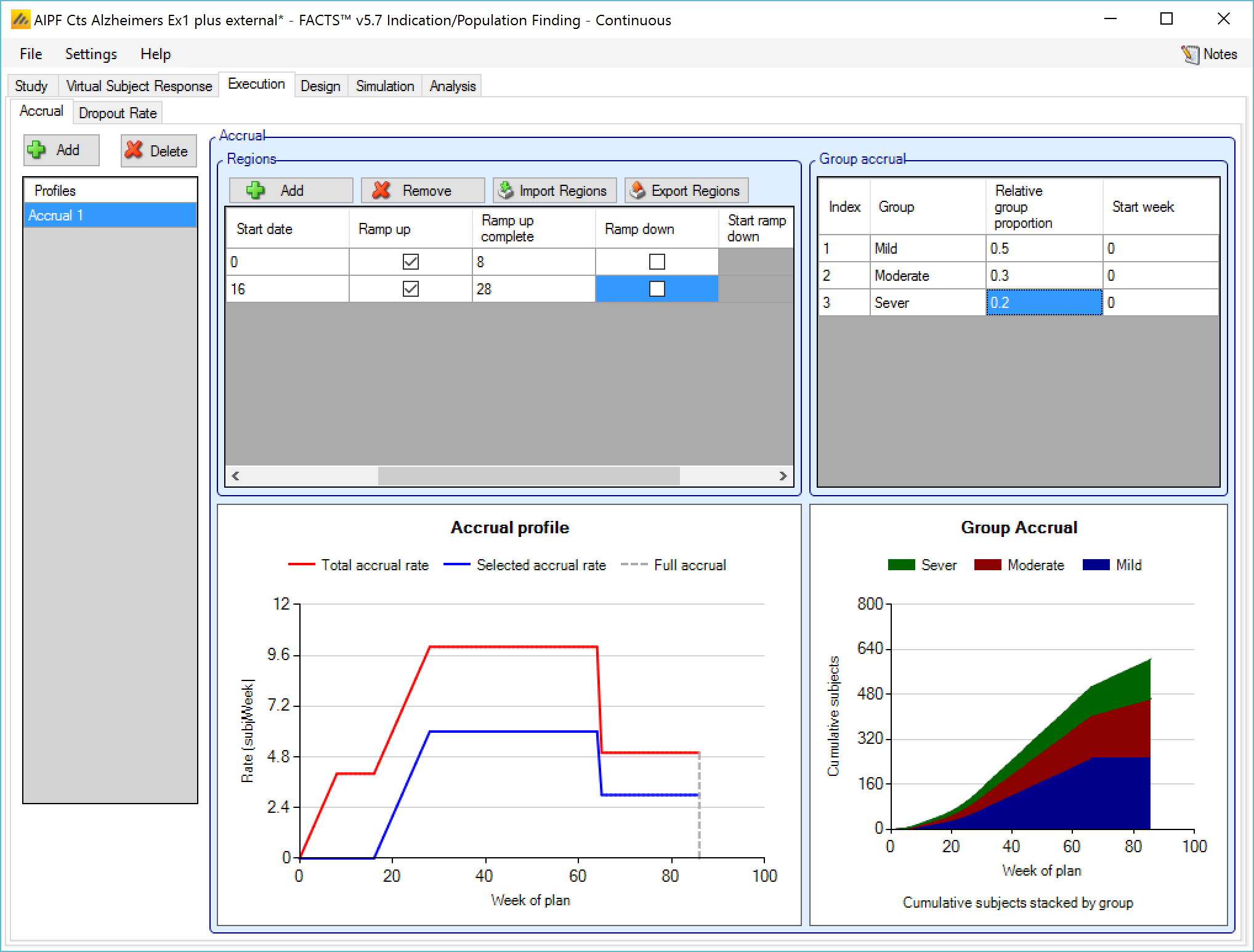
In the screenshot above you can see
The two step ramp up in accrual from the two regions – one starting later than the other.
In the group accrual that the mild group (who constitute 50%of the population) will complete accrual first at about week 65.
The overall recruitment shows a drop after about week 65 because after then only the Moderate and Severe sub-populations will be recruited as the Mild subgroup should have reached its cap.
Note that the accrual profile graph is only the mean expectation; actual accrual is simulated using exponential distributions for the intervals between subjects, derived from the mean accrual profile specified here. Thus some simulated trials will recruit more quickly than this and some more slowly.
There are commands to import and export region details from/to simple external XML files. When importing, the regions defined in the external file are added to the regions already defined, they don’t replace them. Import/export allows an accrual profile with a large specification of regions to be copied to another FACTS design by exporting it from this design and importing it into the other.
The simple XML format means that these region definitions could be shared with other software. This is an example of a simple region file defining with 4 regions:
Region 1: has a peak rate of 1 and starts on week 0
Region 2: has a peak rate of 1 and starts on week 4, with a ramp up that completes on week 8
Region 3: has a peak rate of 1 and starts on week 6, with a ramp down starting week 40 that completes on week 50
Region 4: has a peak rate of 2 and starts on week 10, with a ramp up that completes on week 14 and a ramp down starting week 45 that completes on week 55.
<?xml version="1.0" encoding="utf-8"?>
<regions>
<region>
<name>Region 1</name>
<rate>1</rate>
<start>0</start>
<ramp-up />
<ramp-down />
</region>
<region>
<name>Region 2</name>
<rate>1</rate>
<start>4</start>
<ramp-up>
<ramp-complete>8</ramp-complete>
</ramp-up>
<ramp-down />
</region>
<region>
<name>Region 3</name>
<rate>1</rate>
<start>6</start>
<ramp-up />
<ramp-down>
<ramp-start>40</ramp-start>
<ramp-complete>50</ramp-complete>
</ramp-down>
</region>
<region>
<name>Region 4</name>
<rate>2</rate>
<start>10</start>
<ramp-up>
<ramp-complete>14</ramp-complete>
</ramp-up>
<ramp-down>
<ramp-start>45</ramp-start>
<ramp-complete>55</ramp-complete>
</ramp-down>
</region>
</regions>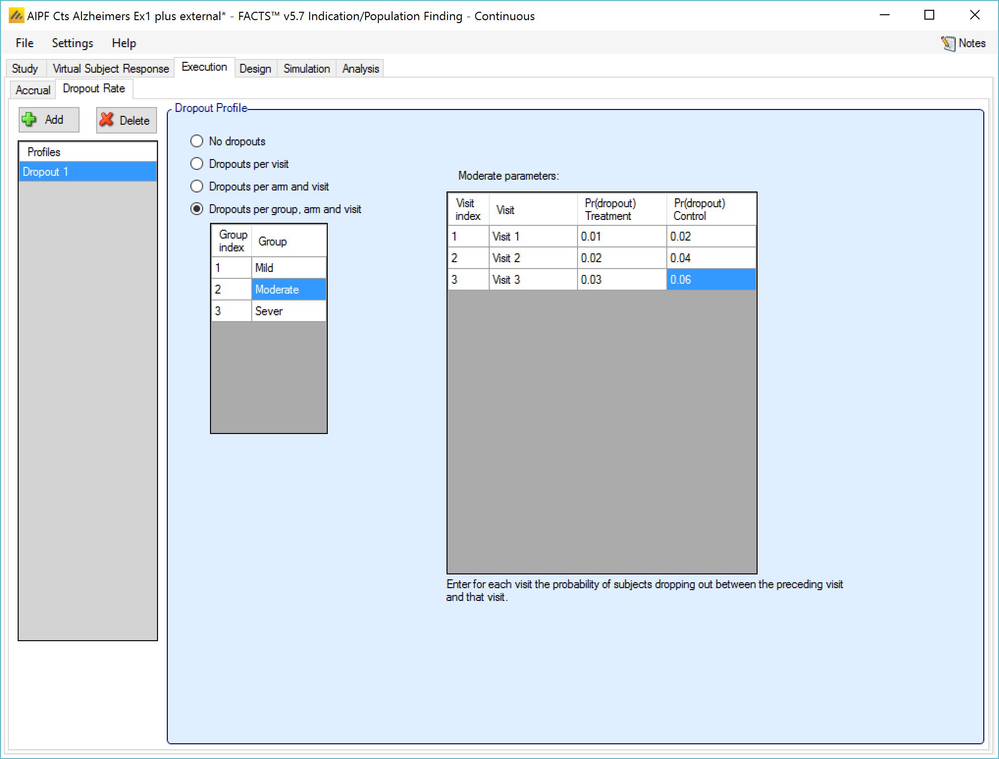
Drop-out Rates
The Dropout Rate sub-tab provides an interface for specifying dropout profiles; these define the probability of subjects dropping out during the trial.
Dropout profiles are listed on the left of the screen, as depicted below. These profiles may be renamed by double-clicking on them, and typing a new profile name. The default dropout scenario is that no subjects drop out of the study before observing their final endpoint data.
The continuous and dichotomous engines allow specification of dropout rate slightly differently than the time-to-event engine.
In the Continuous and Dichotomous engines, the following options for dropouts exist:
- Having no dropout modelling (“No Dropouts”);
- Specifying dropouts as a fraction of all patients per visit (“Dropouts per visit”);
- Specifying dropouts for each arm and visit (“Dropouts per arm and visit”).
- Specifying dropouts for each group, arm and visit (“Dropouts per group, arm and visit”).
Missing Data - A subject that drops out after the first visit will contribute to the Bayesian modeling and frequentist analysis. Final response estimates are imputed based on the completed visits and the selected longitudinal model for Bayesian modeling, and LOCF for the frequentist analysis. However, a subject that drops out before the first visit will be included in subject randomization counts, but excluded from the frequentist analysis and will make no net contribution to the Bayesian modeling. When the longitudinal modeling option has been disabled, no intermediate visits are simulated and for all dropouts the latter approach applies.
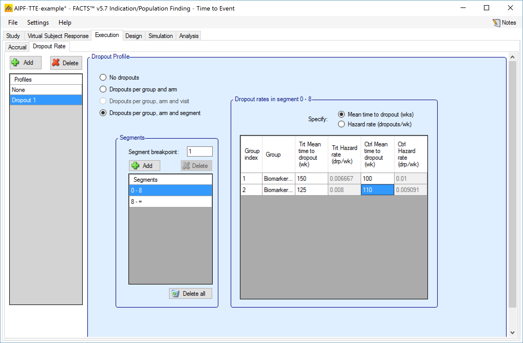
In the Time-to-Event engine, the following options for dropouts exist:
- Having no dropouts included in the simulation (“No Dropouts”);
- Specifying dropouts by group;
- Specifying dropouts by group and visit;
- Specifying dropouts for each group, and segment.
Dropout rates can be specified either by the mean time or a hazard rate (in weeks). When specified by group and segment, a set of dropout specific time segments can be entered; these do not have to match the segments used in defining the control hazard rate (or segments used in the design).
Missing Data – Only subjects that drop out before experiencing an event matter, such a subject’s data becomes censored, contributing only to the overall exposure time.