The Virtual Subject Response tab allows the user to explicitly define virtual subject response profiles, and/or to import virtual externally simulated patient responses. When simulations are executed, they will be executed for a specific scenario – where a scenario is a combination of one each of predictor VSR, control hazard rate, dose response VSR, accrual rate, and dropout rate. If an external file is used to specify the subject responses to be simulated, this effectively replaces the predictor, control hazard and dose response profiles in a scenario.
Unlike other endpoints where just a response (mean change from base line or rate) is specified, specification of subject responses for a time-to-event endpoint is done by first specifying a piecewise exponential event rate for the control population and then hazard ratios for the treatment arms. For simplicity, this means of specifying the simulated event rates is also used when no control arm is present and the comparison is with historic control rates.
In FACTS Core TTE, there is also the ability to include the simulation of a ‘predictor’ endpoint. Predictor endpoints can be a continuous measure, dichotomous outcome, or a precursor event. The interface for specifying how the predictor endpoint data is to be simulated is different in each case.
Specifying VSR with no predictor
Explicitly Defined
With no predictor, there are two screens for defining virtual subject responses; the first is used to define the control hazard rate and the second to define the hazard ratio of the events on each arm to control.
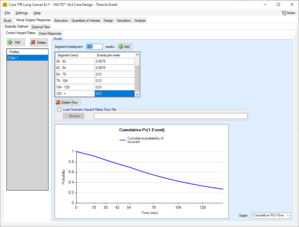
Control Hazard Rates
The user may create a number of different control hazard rate profiles to simulate from. The different profiles will be used to define different simulation scenarios in combination with other profiles defining the other properties that have to be simulated.
The hazard rate to simulate in a profile is specified as a piecewise exponential. The follow-up time can be divided into different time segments and a different event rate simulated in each segment.
Segment boundaries and hazard rates are always entered using “weeks” as the time unit. While this might not always be the most convenient, it allows FACTS to use the same time unit everywhere.
Different segments in the follow-up period are specified by adding segment ends. Adding a ‘segment end’ adds a segment interval to the list to allow the event rate for that interval to be specified. To delete an interval, select the interval starting with the breakpoint to be deleted and click the “Delete” button.
The graph can show the hazard rate, the cumulative probability of not having an event or the probability of not having seen an event over time, using the event rates specified. This is useful for checking that the segments and event rates have been entered correctly.
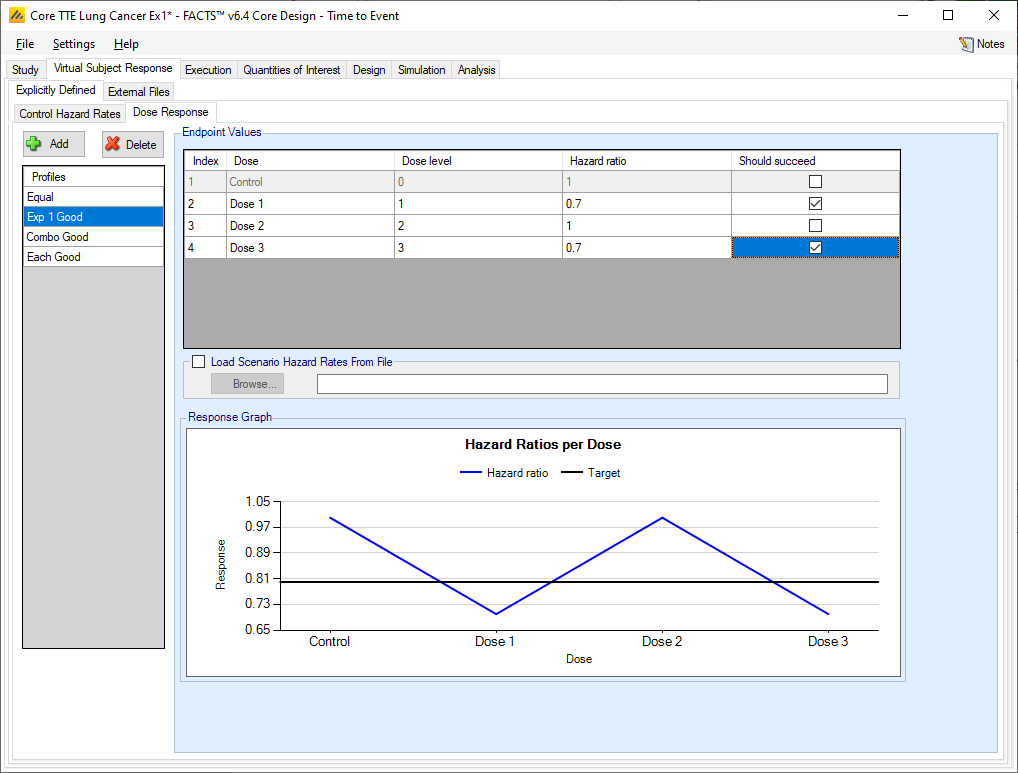
Dose Response
The user may create a number of different dose response profiles to simulate from. The different profiles will be used to define different simulation scenarios in combination with other profiles defining the other properties that have to be simulated.
Within each profile the user specifies:
The hazard ratio compared to control for each treatment arm (except control itself, where of course the ratio is 1).
A check box that allows the user to specify whether a specific arm “should succeed” in that scenario: so that FACTS can report on the proportion of simulations that were successful and a ‘good’ treatment arm selected.
On the graph the different hazard ratios for the profile are plotted, along with the ‘target’ – this is the default CSHRD or NIHRD offset from the QOI tab, the direction of the offset is dependent on whether events are ‘good’ or ‘bad’ and whether the aim of the trial is to show superiority on non-inferiority.
Loading Scenario Control Hazard Rates and Scenario Hazard Ratios from file
If the “Load scenario hazard rates from a file” option is selected then in scenarios using this profile the simulations will use a range of dose responses across the simulations.
Each individual simulation uses one set of responses from the supplied file, each row being used in an equal number of simulations. The summary results are thus averaged over all the VSRs in the file. The use of this form of simulation is somewhat different from simulations using a single rate or single external virtual subject response file. When all the simulations are simulated from a single version of the ‘truth’ then the purpose of the simulations is to analyse the performance of the design under that specific circumstance. When the simulations are based on a range of ‘truths’ loaded from an ‘.mvsr’ file then the summary results show the expected probability of the different outcomes for the trial over that range of possible circumstances. Note that to give different VSRs different weights of expectation, the more likely VSRs should be repeated within the file.
For a TTE endpoint the user must supply 2 files – one for the Control Hazard Rates and one for the Hazard Ratios in each group. MVSR hazard rates are only combined with MVSR control hazard rates. The lines from each file are paired up for each simulation, so the first control hazard rate is used with the first dose response hazard ratio, the second control hazard rate is used with the second dose response hazard ratio and so on. There must be the same number of lines in each file.
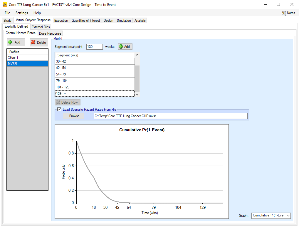
After selecting the “.mvsr” file the graph shows the different control hazard rates over time.
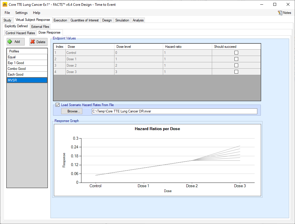
After selecting the “.mvsr” file the graph shows the different individual hazard ratios for each dose.
The VSR parameters are provided in two separate files, (the number of lines in the files should be the same for the two files). The formats are:
Control Hazard Rate File: Each line should contain columns [L1, L2, … , LS] giving the true control hazard rates (\(\lambda\)) for each of the S segments. (Note: FACTS will treat the hazard rate as per week).:
Hazard Ratio File: Each line should contain columns [HR1, HR2, … , HRD] giving the true Mean Hazard Ratios for each of the D dose arms. (Note: HR1 = 1 by definition, but the column of 1’s to be included here for completeness.)
The use of MVSR files has not been extended to the case where a predictor is being used.
External Files
As well as simulating subject responses within FACTS they can be simulated externally and imported into FACTS where the supplied responses are sampled from when simulating the trial. The specification of a file containing subject response data can be done from the External Files sub-tab depicted in Figure 5 below.
To import an external file, the user must first add a profile to the table. After adding the profile, the user must click “Browse” to locate the file of externally simulated data. The user will then be prompted to locate the external file on their computer with a dialog box.
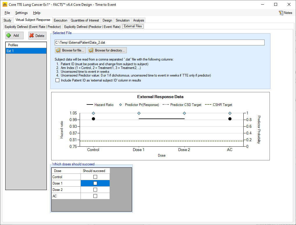
Required Format of Externally Simulated Data
The supplied data should have the following columns:
Patient id, these must be positive integers and unique
Arm Index (1 = Control, 2 = Treatment1, 3 = Treatment2, …)
Uncensored time to event in weeks
This column is a placeholder for predictor data. It may be filled out or empty when there is no predictor. It will be ignored.
The GUI requires that the file name has a “.dat” suffix. The file need not have column headers, but if it does the first column name must start with a pound sign (#) which tells FACTS to ignore that row.
The following shows values from an example file with a dichotomous predictor. Unlike other endpoints there is only one line per subject, as there is no need to record the subject’s state at interim visits.
| #Patient ID | Dose Index | Uncensored Time to Event (weeks) | Optional Predictor value |
|---|---|---|---|
| 1 | 1 | 8.87 | 0 |
| 2 | 1 | 9.34 | 0 |
| 3 | 2 | 6.78 | -9999 |
| 4 | 2 | 10.23 | 0 |
| 5 | 2 | 9.96 | 0 |
| 6 | 2 | 5.6 | 1 |
| 7 | 1 | 37.01 | 20.36 |
| 8 | 1 | 28.67 | 0 |
| 9 | 1 | 39.70 | 0 |
In the above, column headers have been included to make it clearer to read but they are not required.
Simulated subjects will be drawn from this supplied list, with replacement, to provide the simulated response values.
Specifying VSR with a predictor
FACTS supports the specification of the simulation of events and predictors in two ways:
Specification of the predictor and then specification of the subject’s time-to-event dependent on the predictor
Specification of the subject’s event rate and then specification of the predictor dependent on the event rate simulated
Explicitly Defined (Event Rate | Predictor)
The first method (described in this section) may in some circumstances be the more natural way to think of the data (we might want to simulate for instance that subjects with a reduction in tumor size have a longer survival time), however it gives rise to data which does not have an exponential distribution. To retain an exponential distribution in the simulated event rate it is necessary to use the second method where the control rate and treatment arm hazard ratios are specified first and then the probability of the observed predictor derived from that (described in the next section).
Continuous Predictor
If a predictor with a continuous endpoint is being used then there is a new tab in the VSR section to allow the specification of profiles that define how the predictor endpoint is to be simulated.
Predictor
Firstly, the predictor endpoint to be simulated is specified in the same way as a FACTS Core continuous endpoint. A number of profiles can be specified, in each one the mean change from baseline of the predictor for each treatment arm is specified, along with the variability in the change. The variability is specified as the SD of a Normal error in the observed change, a single value can be specified for all arms, or separate values for each arm.
The mean hazard rate for the simulated subjects now depends on the value of the predictor \(Z\), the baseline hazard rate for the time segment \(\mu_{s}\), the log hazard ratio for the dose \(\theta_{d}\), and with parameters \(b_{Zd}\), center and scale for the predictor:
\[h_{sdZ} = \mu_{s}exp\left( \theta_{d} \right)\exp\left( b_{Zd}\frac{Z - center}{scale} \right)\]
Note that in this form of the predictor, the observed event rate is affected by the predictor, it will not be the same as specified in the dose-response profile, also the observed times to event will not be exponentially distributed. The impact of this is best understood by simulating the patient responses and performing rough analyses (e.g. in R).
For example, with a control hazard rate of 0.01, and dose response hazard ratio of 1, when a continuous predictor is added with SD 2, and mean response of 1 on control and 3 on the treatment arm, with center specified at 2, scale at 3 and \(b_{z}\) at 0.2, simulations of 1000 subjects’ times-to-events on each of control and treatment arm give (ignoring censoring) a HR of between 1.05 and 1.21.
Note that if events are bad and higher predictor scores indicate subject improvement (lower hazard rate) then the \(b_{z}\) coefficients need to be negative. The same is true if events are good and lower predictor scores indicate subject improvement.
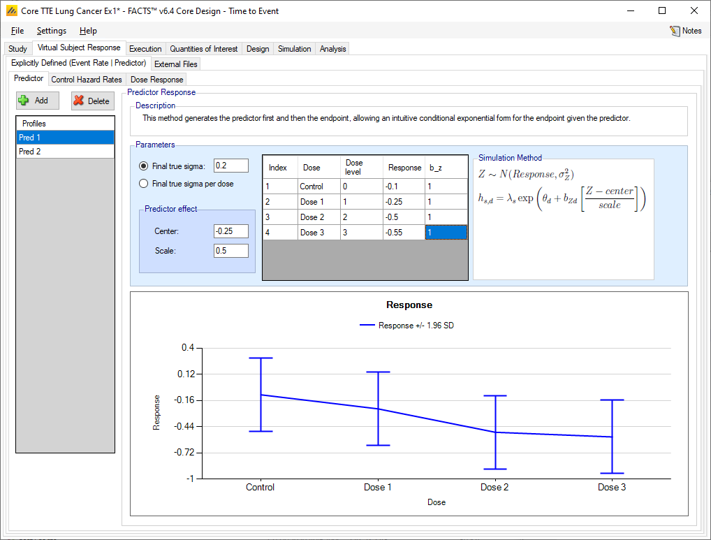
On the graph showing the predictor response to be simulated, the ‘target’ line shows the offset of the predictor CSD from the predictor response on the Control arm.
Control Hazard Rates
With a continuous predictor, the control hazard rate tab does not change. It’s the same as the non-predictor tab.
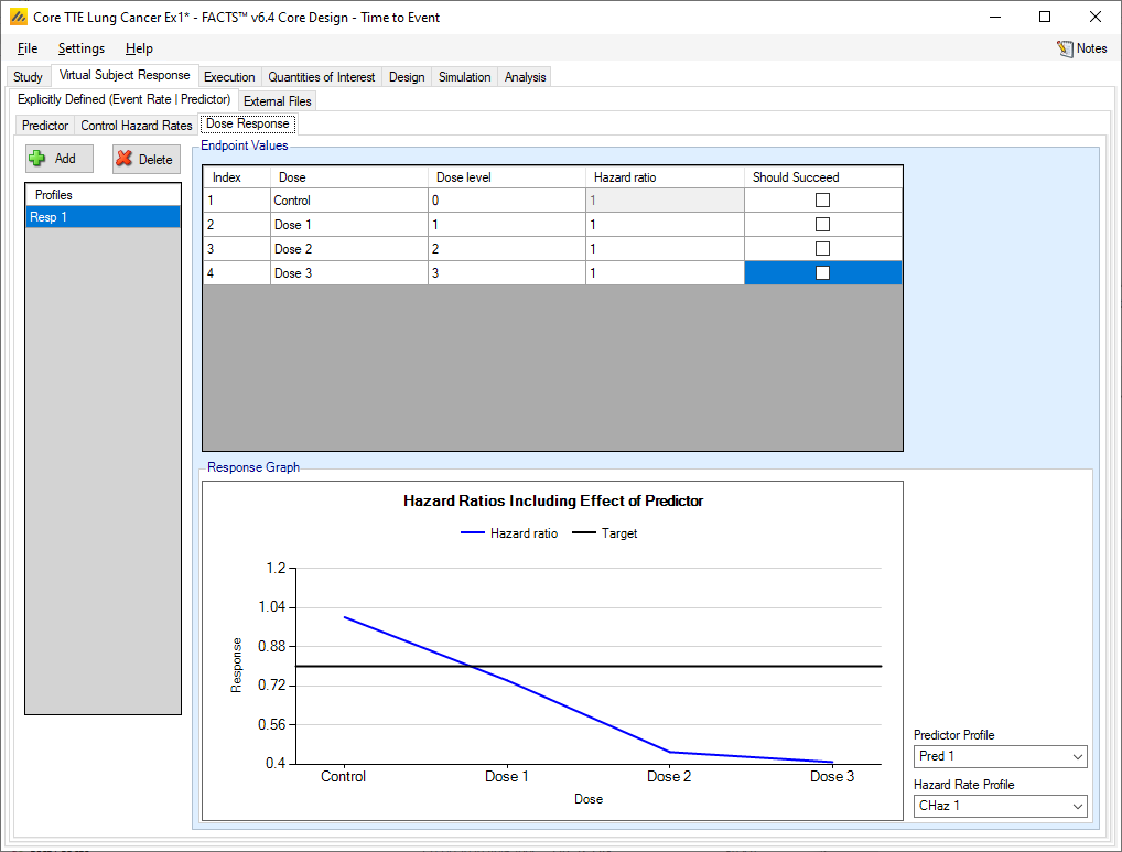
Dose Response
The manner of specifying the dose response does not change – multiple profiles may be specified and in each profile the hazard ratio for each treatment arm is specified. However, the overall hazard ratio simulated will depend on the combination of the control hazard rate, the dose response hazard ratio and the effect of the predictor on the final event rate.
This leads to two different ways for the predictor to be brought into the simulation. First, the hazard ratios \(\theta_{d}\) may all be 1, while the mean of the predictor may change across doses. This would indicate that dose makes no difference given a fixed value of the predictor, but that the different doses achieve their effect by changing the distribution of the predictor values themselves. If the \(\theta_{d}\) values differ from 1, then this indicates that there is a dose effect even conditional on a fixed value of the predictor (thus, for example, a control subject with Z=1 has a different hazard than a treatment subject with Z=1).
The resulting hazard ratio is plotted in the graph at the bottom of the tab. The predictor profile and control hazard rate profile to use in generating the graph can be selected in the controls to the right of the graph.
Dichotomous Predictor
When simulating the event rate conditional on the predictor, the predictor endpoint to be simulated is specified in the same way as a for a simple dichotomous endpoint, the control hazard rate is specified separately for each dichotomous predictor value, and the Dose Response for the time-to-event endpoint has a hazard ratio that depends on the dichotomous predictor’s value.
So, the effect of the predictor on the background event rate is seen on the control hazard rate tab, and on the treatment arm hazard ratios on the dose response tab.
On those tabs the user specifies
separate control hazard rates for subjects who have a predictor response and those who do not
separate hazard ratios for each dose for subjects who have a predictor response and those who do not.
The hazard rates and ratios apply from the moment a subject is recruited (they do not change after the dichotomous predictor is assessed) and do not depend on the predictor being observed (which could be prevented if the event happens first).
The graph shows the specified response rate for each treatment arm and the target rate on control plus CSD.
Control Hazard Rate with Dichotomous Predictor
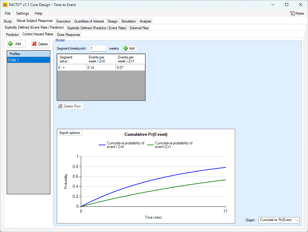
As usual, multiple control hazard rate profiles can be created and the hazard rate on the control arm specified over different time segments. What differs from the case where there is no predictor is that, if a dichotomous predictor (with event rate simulated dependent on the predictor) is being used, separate hazard rates are specified for subjects depending on whether or not they will have the dichotomous predictor response or not.
Dose Response with a Dichotomous Predictor
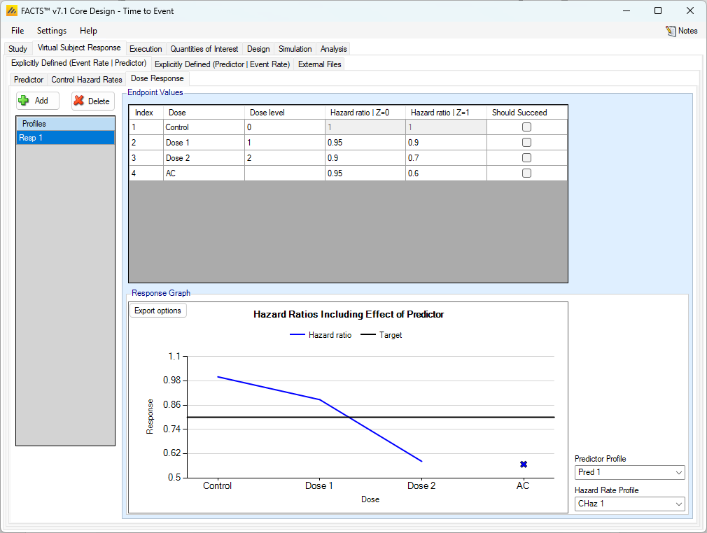
As usual, multiple dose response profiles can be created, and in each profile the hazard ratio to simulate for each treatment arm compared to the control arm is specified. What differs from the case where there is no predictor, is that, if a dichotomous predictor is being used, separate hazard ratios are specified for subjects depending on whether or not they will have the dichotomous predictor response or not.
As with the continuous predictor, the observed event rate is affected by the predictor (it will not be the same as specified in the dose-response profile). Similarly, the observed times to event will not be exponentially distributed. The graph shows the effective combined hazard ratio for a given combination of control hazard rate, predictor rates and dose response. The controls for selecting which control hazard rate and which predictor rates to use are to the right of the graph.
The impact is best understood by simulating the patient responses and performing rough analyses (e.g. in R).
For example, with a predictor response rate on control of 0.1 and control hazard rates of 0.01 (with a predictor response) and 0.02 (with no predictor response), and treatment arm with a predictor response rate of 0.2 and hazard ratios of 0.9 (with a predictor response) and 0.8 (with no predictor response), simulations of 1000 subjects times to events on each of control and treatment arm give (ignoring censoring) a HR of between 0.75 and 0.90.
Time-to-Event Predictor
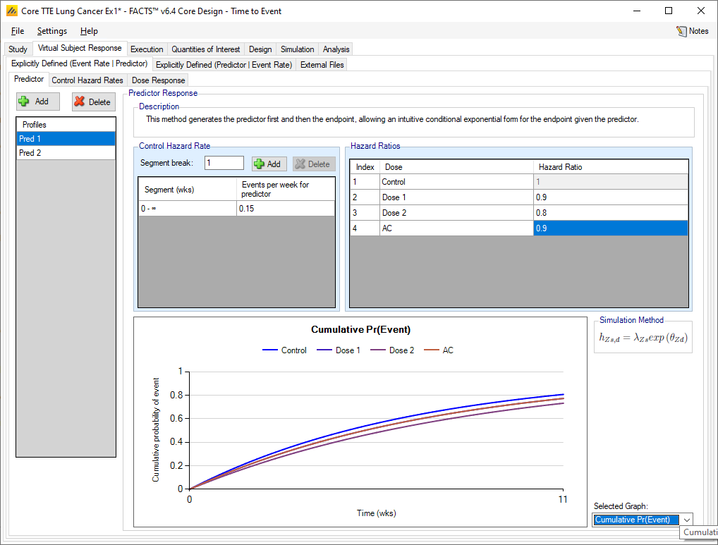
Predictor
The predictor endpoint to be simulated is specified in a similar manner to specifying the simulation of a time to event endpoint. A number of profiles can be specified; in each one the hazard rate on the control arm is specified over one, or more, time segments, and the overall hazard ratio of the time to the predictor event of each treatment arm to the control arm is specified.
The simulation of the time to the final event is in terms of the event rate (over one, or more, time segments) on the control arm after the predictor event, and then the hazard ratio of the time to the final event after the predictor event of each treatment arm to the control arm.
On those tabs the user specifies
separate control hazard rates for subjects post predictor event
hazard ratios for each treatment arm the time to final event, after the predictor event has occurred.
Multiple predictor profiles can be created.
For each profile the control hazard rate can be specified over an arbitrary set of time segments (i.e the time segments can vary from profile to profile, can be different from the observation times (if any) and different from the time segments used in the analysis model.
The hazard ratio of the control arm to itself has to be 1 and cannot be modified. For the other treatment arms, the time to predictor event is specified by specifying the hazard ratio on that treatment arm, to the control arm.
The graph can be used to show the hazard rate, probability of event or probability of not having the event on each arm.
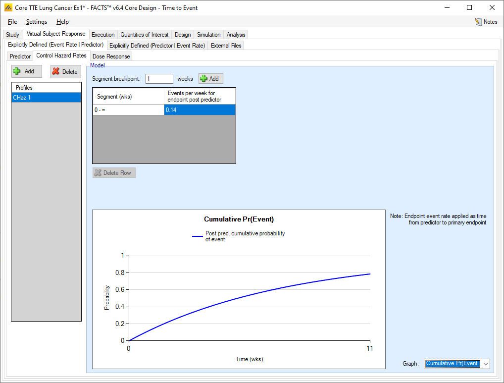
Control Hazard Rates
Specifying the simulation of the control hazard rate with a TTE predictor is the same as specifying the control hazard rate without a predictor. The difference is that with a TTE predictor, the hazard rate specified here is only simulated after the predictor has been seen.
Dose Response
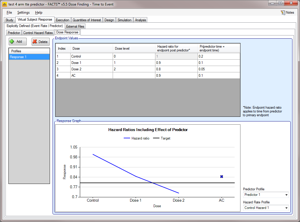
As usual, multiple hazard ratio profiles can be created, and in each profile the hazard ratio to simulate each treatment arm compared to the control arm specified. What differs from the case where there is no predictor is that if a TTE predictor is being used,
the hazard ratios are specified for the occurrence of the final event having observed the predictor event
a probability can be specified that the post predictor event to endpoint event time is 0.
As with the continuous predictor, the observed event rate is affected by the predictor, it will not be the same as the hazard ratio for endpoint post event predictor. The observed times to event will not be exponentially distributed. The impact is best understood by simulating the patient responses and performing rough analyses (e.g. in R).
For example, with a predictor hazard rate on control of 0.1 and post predictor hazard rates of 0.01 and probability that the post predictor event time is 0 of 0.1, and treatment arm with a predictor hazard ratio of 0.9 and post predictor hazard ratio of 0.8 and probability that the post predictor event time is 0 of 0.1, simulations of 1000 subjects times to events on each of control and treatment arm give (ignoring censoring) a HR of between 0.74 and 0.88.
Explicitly Defined (Predictor | Event Rate)
To simulate event times and an associated predictor with a possible correlation between the two in a way that preserves the exponential distribution of the event times, use this tab to specify the simulation of subjects’ time to event first and then the probability of the observed predictor derived from that. This is only supported for Dichotomous and TTE predictors.
The “Explicitly Defined (Predictor | Event Rate)” tab allows the specification of profiles that define how the predictor endpoint is to be simulated in relation to the control hazard rate and hazard ratios for the final events. This allows the simulated final observed final events to still have an exponential distribution.
Once the time-to-event for a subjects has been simulated, a simple user specified transformation of the time-to-final-event provides the expected value of the predictor’s distributions.
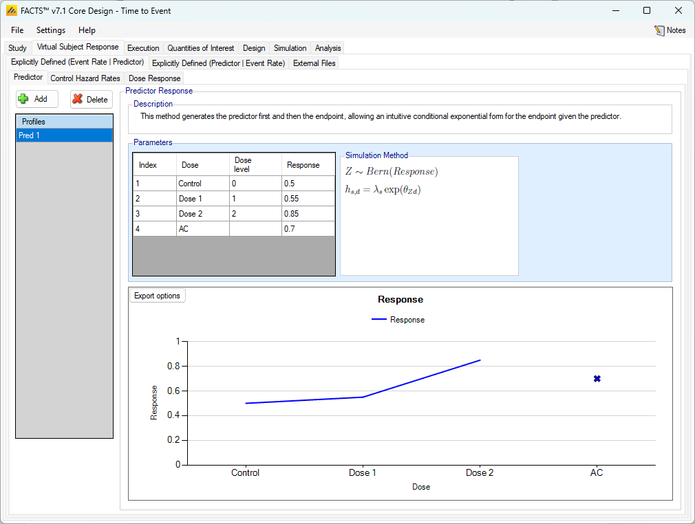
Dichotomous
When using a dichotomous predictor, control hazard rates and dose response hazard ratios are specified as when there is no predictor.
Predictor
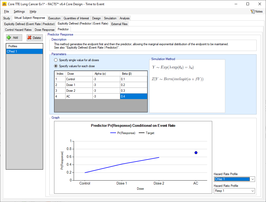
As usual, multiple profiles can be defined. To simulate the dichotomous endpoint given the event rate, the predictor values are simulated by drawing from the Bernoulli distribution with probability given by the inverse logit(\(\alpha + \beta Y\)), where \(\alpha\) and \(\beta\) are specified here and \(Y\) is the subject’s final time to event (in weeks). A single set of values for \(\alpha\) and \(\beta\) can be specified, or separate values per treatment arm can be specified. The expected response rate is shown in the plot at the bottom of the predictor tab.
Time-to-Event
When simulating a time-to-event predictor, control hazard rates and dose response hazard ratios are specified as when there is no predictor.
Predictor
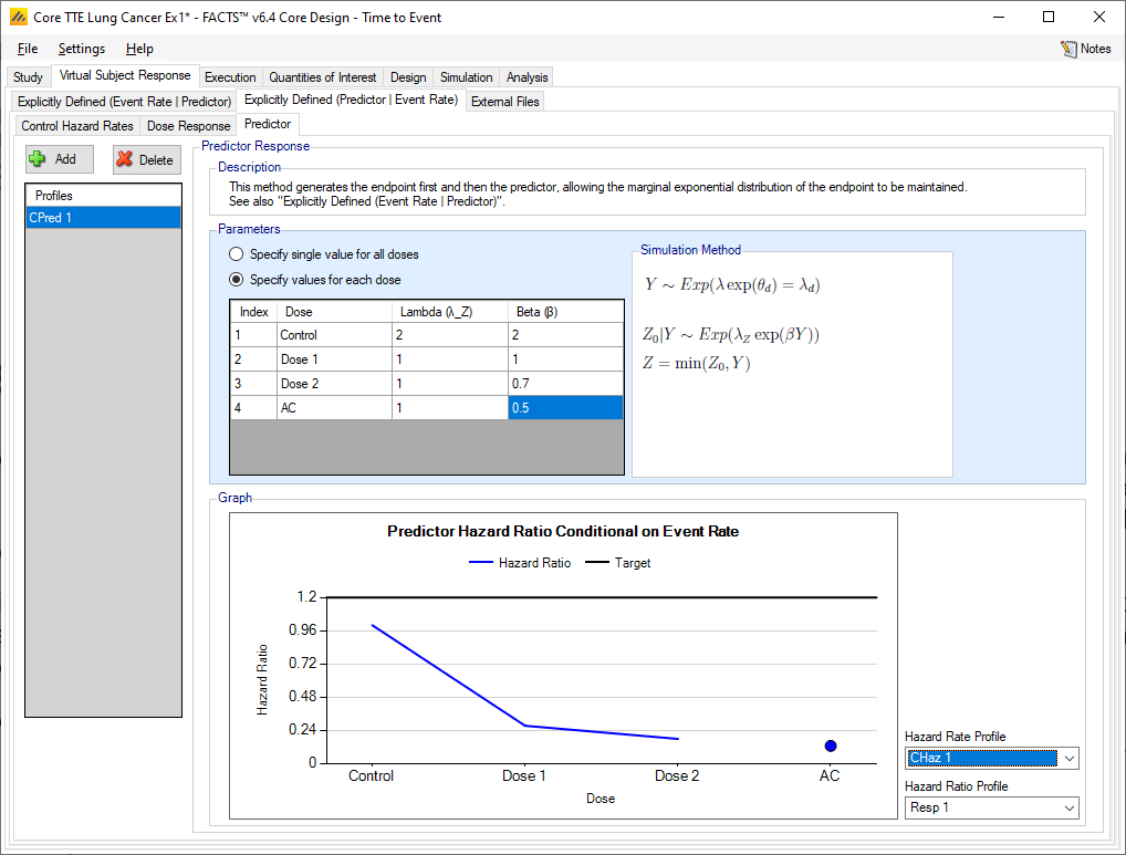
Multiple profiles can be defined. To simulate predictor event endpoint given the event rate of the primary event, the predictor values are simulated by drawing from the Exponential distribution with rate given by (\(\lambda_{z}\exp(\ \beta Y)\)), where \(\lambda_z\) and \(\beta\) are specified here and \(Y\) is the subject’s time to event (in weeks). A single set of values for \(\lambda_z\) and \(\beta\) can be specified, or separate values per treatment arm can be specified.
The arm specific hazard ratios of the predictor given the final endpoint event rate of a specified scenario is shown in the plot at the bottom of the predictor tab. The final endpoint scenario can be changed using the dropdown boxes the right of the figure.
External
As well as simulating subject responses with predictors within FACTS they can be simulated externally and imported into FACTS where the supplied responses are sampled from when simulating the trial. The specification of a file containing subject response data (which must be in the required format) can be done from the External Files sub-tab depicted below (Figure 6‑13).
To import an external file, the user must first add a profile to the table. After adding the profile, the user must click “Browse” to locate the file of externally simulated data. The user will then be prompted to locate the external file on their computer with a dialog box.
Required Format of Externally Simulated Detail
The supplied data should have the following columns:
Patient id, these must be positive integers and unique
Arm Index (1 = Control, 2 = Treatment1, 3 = Treatment2, …)
Uncensored time to event in weeks
Uncensored Predictor value, one of the following depending on the predictor type:
Continuous: “NN.NN” change from baseline
Dichotomous: 0 for no response, 1 for response
TTE: uncensored time to event in weeks
The GUI requires that the file name has a “.dat” suffix. The file need not have column headers, but if it does the first column name must start with a pound sign (#).
The following shows values from an example file with a dichotomous predictor. Unlike other endpoints there is only one line per subject, as there is no need to record the subject’s state at interim visits.
| #Patient ID | Dose Index | Uncensored Time to Event (weeks) | Uncensored Predictor value |
|---|---|---|---|
| 1 | 1 | 8.87 | 0 |
| 2 | 1 | 9.34 | 0 |
| 3 | 2 | 6.78 | 1 |
| 4 | 2 | 10.23 | 0 |
| 5 | 2 | 9.96 | 0 |
| 6 | 2 | 5.6 | 1 |
| 7 | 1 | 37.01 | 0 |
| 8 | 1 | 28.67 | 0 |
| 9 | 1 | 39.70 | 0 |
In the above, column headers have been included to make it clearer to read but they are not required.
Simulated subjects will be drawn from this supplied list, with replacement, to provide the simulated response values.